(1)
Applications of the Hall Plot Method For Monitoring and Prediction of PWRI Performance
Injectivity Monitoring
Whenever water injection is implemented, it is essential to monitor the injection capacity of injection wells throughout the field. This is the case because ultimately any injectivity changes in injection wells can have an effect on the reservoir pressure and the sweep efficiency and therefore the oil production rate. Loss in injectivity can also lead to a need for higher pump capacity, increased workovers or even drilling of additional injection wells. Hence, the economic viability of a development can be highly dependent on injectivity.
Effective injectivity monitoring can give an early indication of any loss in injectivity that is occurring and an indication of the source of the problem. In many cases, this can provide the opportunity to make simple changes in the injection strategy before severe damage occurs.
There are several methods commonly used to monitor injectivity, these include:
Continuous Monitoring of Injection Pressure and Injection Rate – This is the simplest method of monitoring injection well performance. The injection pressure and injection rate are plotted together and any change in one of the variables that is not accompanied by a similar change in the other is likely to be due to injectivity changes in the well. Analysis of such plots can be difficult because of the dual variation of pressure and rate.
Injectivity Index Monitoring – The Injectivity index (II) combines all of the factors that are affecting the injection performance: permeability to water, effective injection zone height, downhole water viscosity, well placement and skin. The monitoring is simple, using measured rate, injection pressure - corrected for bottomhole flowing conditions, and reservoir pressure.
In oilfield units, for radial flow, the injectivity index is presented as:
|
(1) |
A practical disadvantage of injectivity index monitoring is that fluctuations in the measured rates and injection pressure result in a fluctuating injectivity index. Sometimes (maybe usually), the fluctuation is so extreme that it can be difficult to identify real trends. Another disadvantage of strictly using the Injectivity Index is the difficulty of getting a reliable estimate of the effective reservoir pressure (pe) in the vicinity of the well. This may involve shutting in the well on a regular basis to conduct falloff tests. While this is not desirable, it can be a consideration for programmed well shutdowns.
Reciprocal Injectivity Index (RII): This is simply the reciprocal of the injectivity index defined in Equation (1). This index, when plotted against time, is often preferred because it may be less sensitive to inherent operational fluctuations.
Hall Plot Method: This is a technique for continuous monitoring that was developed by Howard Hall in 1963. It is an effective way to process water injection information. The main concept is to plot a cumulative pressure time product against the cumulative volume of water that has been injected. The plot gives an indication of the injection behavior; a change in injectivity appears as a change in the slope of this plot. This cumulative summing reduces fluctuations in the injectivity index. These fluctuations can be due to inaccurate measurements/recording or transient effects caused by operational or reservoir changes. These plots make it easier to identify real changes in injectivity trends. There are various ways of preparing a Hall plot. The theory behind this method, as well as its application, is dealt with in further detail later.
Transient Injection Tests, such as pressure falloff test (FOT) and production logging (PLT) are still important to supplement injection monitoring. Information about the effective reservoir pressure (pe), the effective permeability thickness product (kwhi), skin and fracture behavior (s, xf) can be gained from falloff testing. Effective injection thickness (hi), fracture indications and the number of operating perforations, etc. can be estimated from PLT tests. These tests are often expensive and are therefore usually kept at minimum, but the information gained greatly affects the quality of the injection analysis.
The Theory of the Hall Plot Method
One of the difficulties in analysing injection well performance is the variation in pressure and injection rate with time. The Hall plot method can be used to eliminate complications due to these variations.
This original Hall Plot method is based on Darcy’s equation for radial flow from the wellbore (in oilfield units):
 |
(2) |
where:
qi |
.......................................................... | injection rate (BWPD) |
kw |
.......................................................... | reservoir permeability to water (md) |
h |
.......................................................... | effective formation thickness (feet) |
pbhi |
.......................................................... | bottomhole injection pressure (psia) |
pe |
.......................................................... | effective reservoir pressure (psia) |
| μw | .......................................................... | injection water viscosity at bottomhole conditions |
Bw |
.......................................................... | injection water formation volume factor (often assumed to be 1) |
re |
.......................................................... | distance of the equilibrium pressure from the well center (feet) |
rw |
.......................................................... | wellbore radius (feet) |
s |
.......................................................... | skin factor (dimensionless) |
Integrating Equation (2) with respect to time gives:
 |
(3) |
where:
Wi |
.......................................................... | skin cumulative water injected (BBL) |
The flowing bottomhole pressure, pbhi, can be approximated from the wellhead pressure by using:
(4) |
where:
pwh |
.......................................................... | wellhead pressure (measured) |
| Δpf | .......................................................... | frictional pressure drop in tubing and completion |
| ρg x TVD | .......................................................... | hydrostatic head of fluid to midpoint of perforations |
Substituting Equation (4) into Equation (3) and rearranging to separate the wellhead pressure term gives:
 |
(5) |
If the effective reservoir pressure, friction and the hydrostatic head are assumed to be constant with time and numerical approximation is used, Equation (5) becomes:
 |
(6) |
In Equation (6),ξis a constant. This is a linear equation. A plot of the cumulative volume injected (Wi) versus the pressure summation (the left-hand side of Equation (6)) gives what is known as a Hall Plot.
Simplified Hall Plot Method
It is a common (but often inappropriate) simplification to plot only cumulative wellhead pressure against cumulative volume, and ignore the last part of Equation (6):
(7) |
This has the advantage that only variables directly measurable at the surface; wellhead pressure and injection rate, are needed.
It must be must be appreciated that this equation is not mathematically correct. Therefore, the slope of the simplified Hall plot is skewed and no longer has a quantitative meaning (such as RII). Still, changes in injectivity will appear as changes in the slope and the plot can be useful to approximately identify injection well behavior.
The Modified Hall Plot Method for Radial Flow into Vertical Wells
As stated earlier the simplified versions of the Hall plot method have some important limitations:
In modern computer environments, it is not complicated to adjust the available pressure information to bottomhole conditions, by adding on hydrostatic head and subtracting the correct tubing and perforation friction and reservoir pressure. The modified Hall plot method is based on plotting the injection pressure potential {∫(pbh- pe) dt} against the cumulative injection, Wi.
| (8) |
This relationship is mathematically correct and therefore, misinterpretations are less likely to occur and the slope of the plot has a real physical meaning:
| (9) |
This is indeed an average value for the reciprocal injectivity index.
The Hall Plot Method for Horizontal Wells
The Hall plot method also works for horizontal wells, except that the slope has a
different meaning. The inflow can no longer be assumed to be radial and the slope will represent a more complex geometry. From Joshi´s equation for horizontal wells the slope can be derived as (use whichever analytical approximation of horizontal injection that you prefer):
| (10) |
where:
kh |
.......................................................... | horizontal reservoir permeability |
kv |
.......................................................... | vertical reservoir permeability |
Sfd |
.......................................................... | skin factor for formation damage |
The Hall Plot Method for Fractured Wells
Most water injection wells are fractured, either intentionally or by means of thermally induced fractures. The Hall plot method is also valid. Remember, however, that you will need to incorporate skin into the radial flow equation (as in Equation 2) for quantification of the effect of the fracture. In fact, the Hall plot does offer a means of quantitatively determining skin and changes in skin by manipulating the basic equations.
The Meaning of the Hall Plot Slope
Figure 1 illustrates a Modified Hall Plot with several changes in slope accompanied by possible explanations for the well injectivity changes.
Figure 1. A characteristic modified Hall Plot, showing fluctuations due to the type of fluid (influencing bottomhole formation face pressure and mobility) and an acid treatment. This slope is governed more by viscosity than by stimulation.
Buell et al. stated that, in order for slope changes on the Hall Plot to be correctly interpreted the reservoir pressure must be included, i.e. the Modified Hall Plot must be used. Figures 2 and 3 are examples of the impact of not only incorporating the reservoir pressure but incorporating temporal variations in the pressure.
Figure 2. This shows the average reservoir pressure in the regime affected by an injector – in a chalk. This reservoir pressure was determined by simulation. Figure 3 shows the consequences of not accounting for the reservoir pressure variation.
Figure 3. This is a dramatic illustration of not using the actual reservoir pressure (Figure 2) in the Hall plot calculations. If you assume a constant reservoir pressure, you can make some erroneous decisions. You would look at the increasing slope of the curve and say that this reservoir is being damaged substantially. In fact, if the actual (and varying) reservoir pressure is used, injectivity is seen to be actually improving. That does not mean to say that there are not issues – likely associated with fillup.
The Modified Hall Plot may be used as a monitoring tool to identify problem injectors. It may also be used to evaluate the effectiveness of a stimulation treatment or to compare the effectiveness of several stimulation treatments against one another (refer to Figures 4 through 7).
Efforts have been made to use Hall plots more quantitatively for the evaluation of the effectiveness and longevity of stimulations. This is using an improvement index, which shows the ratio of the II after and before stimulation and – from the date of the stimulation extrapolates the behavior from immediately after the stimulation forward in time. When deviation from this extrapolation occurs, there is an indication that supplementary stimulation is required (Figure 7).
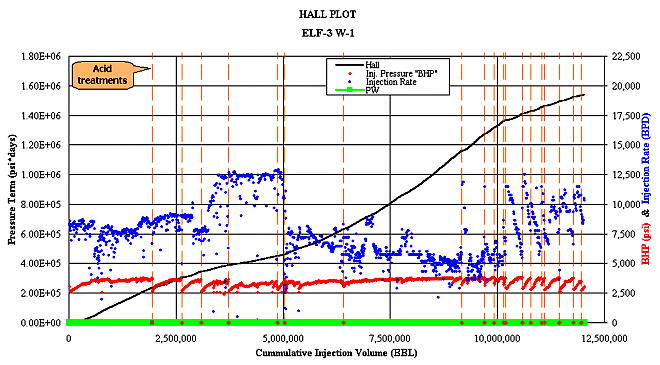
Figure 4. This Hall plot indicates the use of Hall plotting for inferring injection improvements. A reduction in the slop indicates improved injectivity. It can be seen that the frequent acid treatments – although expensive – did improve injectivity – although their individual impact was relatively short-lived.
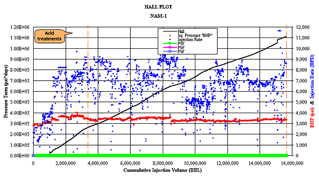
Figure 5. This Hall plot indicates improved injectivity after about 4,000,000 bbl or injection. It was speculated that this might have had more to do with the well being fractured at that time rather than the acid treatment. In fact, this is maybe seen better by looking at the following figure (this indicates one of the drawbacks of standard, modified Hall plotting in that the averaging effects are very large). All available information must be used together!
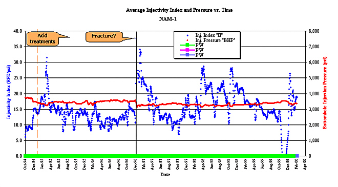
Figure 6. This figure substantiates the inferences made in the previous figure that fracturing probably led to improved injectivity. Substantial other analyses on this well have indicated that it probably did fracture.
Figure 7. This figure shows the recorded Hall Plot and an extrapolated brown line showing how the ideal plot would look if the performance immediately after a stimulation was “maintained.” You can see upward deviation from this trend (damage) and you can infer information on the required frequency of a particular type of stimulation.
Summary
The main advantage of using this method for injectivity tracking is that the required data are usually readily available.
In addition, a continuous monitoring system over a period of time is provided which can be more representative of trends than single point measurements from a falloff test, for example.
The Hall Plot Method is totally reliant on accurate flow meter and pressure gauge measurements and a reliable method to convert WHP to BHP.
Another difficulty is that in order to use the Modified Hall Plot an estimate of effective reservoir pressure variation (re) over time is required. This may not always be available. In reservoirs with very good connectivity (high permeability homogeneous) the reservoir pressure may be well defined, but in tight reservoirs, it may be more difficult to infer the pressure variation.