Tuesday March 27, 2001
Attendees
|
Ahmed Abou-Sayed |
Advantek |
Brian Odette |
First Choice |
|
Marco Brignoli |
AGIP |
Henrik Ohrt |
Maersk |
|
Roberto Cherri |
AGIP |
John Shaw |
Statoil |
|
Jean-Louis Detienne |
TFE |
Alastair Simpson |
Triangle |
|
Marc Hettema |
Statoil |
Idar Svorstol |
Norsk Hydro |
|
Trond Jensen |
Phillips |
Paul van den Hoek |
Shell |
|
Bruce McIninch |
Marathon |
Dale Walters |
Taurus |
|
John McLennan |
TerraTek |
Karim Zaki |
Advantek |
|
Laurence Murray |
BP |
|
|
Overview Session
Marco Brignoli welcomed the
participants and outlined safety and organization details. John McLennan summarized the agenda and the financial
status of the Project.
The purpose of the meeting was
indicated as:
Ø To review
ongoing contractor work and to critique planned activities.
Ø There
will be a summation of results from each Task (on Tuesday, 3/27) followed by a
Task-by-Task presentation of gaps, future requirements, and recommendations for
ongoing work on Wednesday, 3/28.
Ø Thursday
morning, 3/29 is set aside for a Sponsors review, followed by feedback to the
Contractors.
Ø Thursday
afternoon will be the start of a workshop on the Toolbox, which will continue
through Friday morning for a tentative adjournment before lunch on Friday
morning.
The Sponsors reviewed the
financial status. The only question
raised was what has happened to interest on the money that has been
provided. This question was posed to
Bob Siegfried, with GTI, and his response is as follows.
John-
I have asked our attorney to review the PWRI sponsor agreements regarding
the accrual of interest on funds collected for the project. His reply is
excerpted below:
Section 4.4-b provides the following: "In the event that more than sixteen
(16) Sponsors join the Project, a proportionate share of the excess
contributions shall be repaid to the Sponsor upon Project Completion or
termination. However, the Steering Committee ... by vote approval may
decide to increase the total budget of the Project as long as this does
not imply major changes in the scope and objective." Because there is no
provision in the contract for the payment of interest on excess funds
collected, normal rules of contract construction will not imply one. The
parties only stipulated upfront that excess contributions will be
"repaid"
on a proportionate basis (without reference to interest on such funds).
Thus, while we will cooperate fully in the establishment of a new
administrative arrangement and return excess contributions to the sponsors
as provided in the agreement, we do not plan to pay interest on these
funds.
Regards,
Bob
Robert W. Siegfried, II
Gas Technology Institute
1700 South Mt. Prospect Road
DesPlaines, IL 60018-1804
(847) 768-0969 Fax: (847) 768-0995
Robert.Siegfried@gastechnology.org
Overall Summary of Tasks
John McLennan provided a brief
overview of the status of all of the Tasks. The slides in the presentation are
self-explanatory. There are some
remarks that are relevant.
- For all Tasks, Paul van den Hoek emphasized
the importance of providing reports that, for example, discuss what was
done when data were analyzed.
- Jean-Louis indicated that it was necessary to
check the links to the files in the Workshop.
- Task 1: In discussions of falloff testing,
indicate why don’t commercial software simulators work. What are their limitations and what is
the range of validity?
- Jean-Louis Detienne
(shortly after the meeting) provided additional information on fracture
models being used at TFE (Hydfrac, Diffrac, and Predictif). These have been added to the model
audit document for Task 1 and will be distributed for review soon.
- Task 3: Various changes in the Completions
Worksheet are being made based on observations by Laurence Murray and Paul
van den Hoek.
Task 1 – Monitoring
John McLennan provided more
detail on Task 1, covering Monitoring
and Interpretation. The key elements of
the presentation are as follows.
- John indicated the status of incorporating
monitoring methods in the Best Practices document. The status is:
Ø
Conventional methods completed
Ø
Need to add fiber optics
Ø
Need to finalize PLTs
Ø
Need to improve fractured
monitoring
Ø
Need to incorporate specific Best Practices, in addition
to the descriptions of the various methods.
Ø
Falloff testing was discussed (Slides 3 and 4).
Ø
Slide 5 describes the importance and analytical methods
for determining average pressure. It is
emphasized that even if these evaluations are done with software it is
desirable to understand the basic principles and the potential pitfalls.
Ø
Slide 6 outlined the status of the section on Hall
plotting. Basic documentation is done
and additional information is being added on some of the moving average
concepts that have been recently developed.
Ø
Step rate testing and Hydraulic Impedance testing have
been completed. Sections have been
added on pulse testing, interference testing, leakoff testing and
micro-hydraulic fracturing. The section
on Drillstem Testing will be brief as it is discussed in detail in numerous
public domain references.
Ø
Prior to the meeting, sections were added on tiltmeter as
well as microseismic monitoring.
Ø
Real-time methods for evaluating the success of acidizing
have been included in the Best Practices.
Ø
The status of the Fracture Modeling Audit was reviewed. As indicated, some recent additions have
been made (TFE models and additional information on two Shell models).
Ø
Because of its relevance, a brief section describing some
of the key theoretical aspects of evaluating well performance (with a focus on
injectors) has been started and will be completed before June.
Ø
The new look of the Best Practices document was
presented. The philosophy is to
navigate on the basis of appropriate well or field activities rather than
according to Tasks in the JIP.
Tasks 2 and 4
Tasks 2 and 4 cover Matrix Injection and Stimulation/Mitigation, respectively. Because of commonality in these Tasks, they were presented together by Ahmed Abou-Sayed. Ahmed prefaced his discussion by showing the contents of the Toolbox, as it currently stands and summarizing the planned modifications (additional modifications were specified by Sponsors as the Meeting went on).
Ahmed continued with a
presentation on Matrix Injection issues.
Recall that matrix injection has been specified to include injection
into non-propagating fractures. Some of
the observations made included the following:
1.
The Reciprocal Injectivity Index –RII, following on from
Chevron's use of this, has been adopted for many of the analyses that are
carried out. Paul van den Hoek wanted to know why was RII used rather than II.
2.
A number of examples were given as to the influence of
reservoir pressure – constant versus variable.
The basis for the analyses were wells from two blocks in the Maersk A
field. Reservoir data are imported into
the Toolbox for analysis. Ahmed
committed to allow reservoir pressure to be interpolated between discrete
chronological measurements to represent approximations of temporal variation in
reservoir pressure.
3.
Ahmed then showed a Phillips' field case in a chalk. The reservoir pressure was determined from
history matching (Figure 1). Figures 2
through 4 illustrate, fairly dramatically, the pitfalls of not using the
correct reservoir pressure. Figure 2 is
a Hall plot. The two curves are bases
on 1) constant reservoir pressure and 2) the reservoir pressure shown in Figure
1. Certainly constant reservoir
pressure assumption, in this case, would be misleading. Figures 3 and 4 support the observations in
Figure 2 on the basis of the variation of the Reciprocal Injectivity
Index. Some actual injectivity
improvement is seen if a variable reservoir pressure is incorporated (this may
actually be a situation where some fracture growth is occurring?).
Figure 1. Reservoir
pressure in an example chalk well, chronological.
Figure 2. Hall plot determined with a constant reservoir pressure and with the reservoir pressure shown in Figure 1. Certainly the assumption of constant reservoir pressure could lead to costly and unnecessary intervention.
Figure 3. The variation of the Reciprocal Injectivity Index with date, calculated presuming that the reservoir pressure was constant. The increasing RII plotted would mistakenly indicate loss of injectivity (see Figure 4).
Figure 4. The variation of the Reciprocal Injectivity Index with date, calculated using the reservoir pressure from Figure 1. The increasing RII plotted would seem to indicate relatively constant injectivity (see Figure 3).
The next topic discussed was
modifications to the Frictional Calculations Program that are planned
(additional changes were suggested to Karim Zaki when he presented the Toolbox
itself, later in the week - for example, multiple tubing strings and a way to
include minor losses - e.g. valves).
Ahmed indicated that they were adding viscosity changes with
temperature, density, and viscosity, as well as the influence of solids content
on viscosity. The rationale for this
level of sophistication was a point of argument, presuming that roughness will
have a large role. However, it was
accepted that any level of improvement in BHP inference was important because
the net pressures (either above closure or above the formation pressure) are
often quite small.
Next a series of slides was shown to demonstrate characteristic differences between matrix and fractured injection. There was the Elf3 example, under matrix injection – there was one step where there was no propagation of a fracture. This was followed by a Shell NAM example showing some spontaneous fracture growth events and a BP Prudhoe Bay example. There was a great deal of consternation because the slides were labeled as indicating that there was stimulation. NOTE: The use of the word stimulation. In the context of these slides stimulation refers to improved performance because of spontaneous fracture growth, as well as hydraulic fracturing or acidizing.
Finally, there was emphasis of
the concept that fractures are conductive even when they are nominally
closed. Fractures are conductive long
before they are reopened. Ahmed showed
a plot from Voegelle et al., 1982, based on large block testing that showed
fracture conductivity even with high normal stress, acting across pre-existing
fractures. Roberto Cherri and Ahmed
discussed this concept at some length.
Ahmed next discussed some of the
recent work that has been done on Task 4 - Stimulation. The premise was a mechanism for sporadic propagation
of a fracture after it had been progressively plugged. Signatures for this were indicated on RII
plots. Figures 5 and 6 are examples of
the concept. In these figures, it was
suggested that the upper locus (blue line) is largely controlled by
temperature, damage and pore pressure, whereas the lower locus (blue line) is
mostly impacted by the in-situ stress conditions. Figure 7 shows further specifications. All of the slopes shown can be taken to be diagnostic. In Figure 7, the rate of change during the
plugging phase is a function of the water quality and the amount of recovery in
RII after fracturing is governed by the in-situ stress conditions.
Figure 5. The variation of the Reciprocal Injectivity Index with time. RII varies between two loci. The fracture plugs, the injectivity declines. The pressure increases until finally some supplementary fracture extension spontaneously occurs and new injection surface area and fracture volume is created.
Figure 6. The variation of the Reciprocal Injectivity Index with time. RII varies between two loci. The fracture plugs, width may increase but length growth is impeded and the injectivity declines. The pressure increases until finally some supplementary fracture extension spontaneously occurs and new injection surface area and fracture volume is created. This figure goes one step beyond Figure 5. It is an assertion that when the two blue loci intersect complete plugging occurs and injectivity will be largely lost unless a completely new fracture system is created.
Figure 7. It is believed that the slopes in this type of RII plot can be diagnostic. For example, you will want to stimulate before the two blue loci intersect. The specific slopes are functions of certain controllable and uncontrollable parameters.
It is hypothesized that this
type of plot can provide real diagnostic information on when stimulation should
be done. For example:
1.
When the lower blue locus (the minimum fracturing
pressure) intersects the upper locus, the fracture is completely filled and
there will be a dramatic rise in pressure. Figures 8 and 9 are examples. Figure 10 suggests another presentation of
such data (in a step rate type plot).
2.
Stimulation can be planned by establishing the two loci,
predicting their intersection and ensure that you stimulate adequately in
advance.
3.
If the loci are relatively parallel (the Prudhoe Bay
example in Figure 11), explicit intervention for artificial stimulation will be
required relatively infrequently.
4.
The lower locus for RII corresponds to matrix injection in
a stationary fracture. Upper bound is
fracture injection. The bottom and top
loci can be parallel.
5.
Both lines could reflect matrix injection, one is clean
one is dirty.
6.
It is desirable to tune these lines.
7.
If the two lines intersect, you have no tolerance for a
drop in pressure. When the two lines
come together, it means you must propagate a fracture for further accommodation
of solids. You must be able to
accommodate the fluids. You need to
decide when to stimulate.
8.
The upper line is governed by the stress and the lower
line governed by the damage - or is it the other way around as was shown in the
slides. There was some argument that
the filter cake should be attached to the bottom line.
9. RII for
a fractured condition needs to be based on the pressure minus the fracture
propagation pressure.
The next issue that was
addressed was the validity of the PEA-23 correlation outside of domains similar
to Prudhoe Bay. How can PEA-23 be extrapolated outside of Prudhoe Bay? It was argued that this requires a method
for predicting frac gradient. Ahmed
speculates that PEA-23 behavior will be seen if propagation occurs before the
fracture is too fully filled.
An example from the Maersk A
field was used for the assessment.
Ahmed then discussed an approach for using these observations as a
diagnostic tool. A baseline RII was
defined, indicative of best performance for a well. Certain other terms were also defined. These included slopes of the RII plot before and after
stimulation and DRIIbefore and DRIIafter (before and
after stimulation). These are the
deviation of the RII from the baseline before and after stimulation. DRII is a measure of damage and the slope of
the RII plot is an indication of the rate of damage accumulation.
Once you go past the
intersection of the two blue loci, you cannot go back to the baseline. What you create with stimulation may be
embedded in the damaged zone?
Figure 8. Progressive plugging is hypothesized for this well along with break-back as new fracture area is created or accessed. If you draw bounding loci for this situation they would seem to diverge, suggesting interpretation can be more complicated than envisioned. On the other hand, Figure 9 tends to support the validity of the locus construction method.

![]()
Figure 9. Without too much imagination, two bounding loci can be drawn. When they intersect, significant loss in injectivity is indicated and presumably the recourse at this time was stimulation.
Figure 10. Step rate type presentation showing stationary fracture (blue), propagating fracture (red) and a plugged fracture in yellow.
Figure 11. This is an example from Prudhoe Bay where relatively little human intervention is required. The fracture system sporadically extends but the two loci are relatively parallel. The behavior at the end was attributed to shutdowns.
Two examples of looking at the
slopes and the DRII are available in the presentation. An Improvement Ratio was defined as the DRIIbefore/DRIIafter.
Note:
You need to have enough pressure capacity in your system to be able to handle
the events. It is a discontinuous
rather than a continuous process - discontinuously propagating fractures - a
self-correcting process.
In the
long run, even if you have enough pressure available, you may not be able to
stimulate adequately.
There was further discussion of
the meaning of the various slopes.
Laurence Murray discussed water quality as a regulator for the
"red" slope. Why does the red
line commonly have a constant slope? If
the water quality changes, the slope changes for the red lines. Laurence believes that you can argue that
propagation is not the only mechanism for cleanup and that change in water quality
is another one. The red lines can be
extracted from PEA-23.
What are some of the products of these concepts? One example is an extension of PEA-23 with
time, the influence of water quality on the frac gradient, and looking at the
influence of tortuosity (per Paul van den Hoek).
After Paul brought up tortuosity there was additional
discussion. Laurence Murray supported
the role of near-wellbore effects (citing three distinct data sets for produced
water injection and oriented perforations where pressure loss was
systematically determinant). Jean-Louis
Detienne supported the importance and argued for additional consideration of
the completion skin.
Task 3 – Soft Formations
Dale Walters summarized the
status of the Task on Soft Formations. The relevant components of Dale’s
presentation are as follows:
- Work completed since the December Meeting in
Houston is:
Ø Additional
data for soft formations has been received since the December 2000
meeting. This includes two Brage wells
and Heidrun pilot data. An example of
the Brage data is shown in Figure 12.
Figure 12. Injection
data from one of the two Brage wells being evaluated currently. There are also SRT results (Figure 13).
Figure 13 shows step rate test data for one of the new
wells. These data will be useful
because there is both produced water and seawater injection.
Ø Further
improvements have been made to the radial damage spreadsheet analysis tool
(Jean-Louis Detienne has suggested that this tool should be called PWRAD) based
on Dec 2000 meeting (isolating completion skin). A User Guide has been written.
The
completion skin is now input separately, following discussions of the Kerr
McGee G field data at the December Meeting in Houston. Those data have been reanalyzed, assuming a
completion skin, Sc, of between 100 and 250. The skin due to damage is predicted to be
smaller but still significant (Figure 14).
Figure 14 shows skin of 600± during
later phases of the injection.

Figure 13. Step rate test data from one of the Brage
wells. This data set is “nice” because
it has both seawater and produced water injection information.
Figure
14. PWRAD simulation for a well in
Kerr McGee’s G Field, showing the position of the water front, the calculated
permeability in the flooded zone and the skin.
Figure 15 shows better-sustained performance in an
equivalent BP Amoco Field. Specific reasons
for this have not as yet been determined.
Figure 15. The injectivity index for two wells in the
G field and an equivalent BP Amoco well.
Ø
The injectivity index for two wells in the G field and an
equivalent BP Amoco well.
Ø
Re-analysis of all data sets with the modified tool and
assessment of the differences, with inputted values for the completion
skin. There were no substantial changes
in the conclusions.
Ø
A tool entitled WellStress has been developed and is
available in the Toolbox. This is a poro- and thermoelastic stress evaluation
tool. A User Guide has been written.
Ø
Corrections and revisions have been made to the reports
issued for December meeting
Ø
Evaluation of injectivity of various completions has
continued.
- Dale then described work in progress,
scheduled to be finished before the end of June. This includes the following:
Ø No new
data analysis will be undertaken.
Taurus suggested including the Brage and Heidrun pilot data analysis in
a project extension? The SRT will be
incorporated in Task 1 (Monitoring).
Ø A report
will be prepared on the completed Soft Formations (SF) data analyses. This will include the general methodology, a
detailed discussion of each data set, findings from the comparative analysis,
and, a concise summary.
Ø Investigate
if a PEA 23 type correlation for fracture injection mode is feasible in soft
materials.
Ø Write a
User Guide for the Radial Damage Tool
Ø Summarize
Task 3 results. This would include major
learnings, concepts, developments; gaps in understanding; future work that may
be needed and Best Practices.
- Taurus also provided some suggestions for
appropriate future developments/efforts.
These included:
Ø Develop
a comprehensive Completion Skin Tool for inclusion in the Toolbox - full set of
correlations for cased and perforated completions, correlations for screens,
liners and excluders …
Ø Analysis
of newly-arrived data sets (Brage, Heidrun pilot)
Ø Rewrite
WellStress library (portability)
Ø Improvements
to PWRAD.
More will be said about future efforts later in these
minutes.
Task 5 – Layered Formations
John McLennan summarized the
status of the Task on Layered Formations.
Ø The
first two slides in the presentation emphasized that even for matrix injection,
analytical methodologies are difficult to use when there is crossflow. Specifically:
ü Without
a simulator, it is difficult to represent interlayer vertical crossflow
ü However,
for horizontal crossflow on shut-in, there is an analytical tool that is
available in the ToolBox. A Users’
Guide is being prepared.
ü Methodologies
for minimizing horizontal crossflow have been encapsulated in Workshop minutes and
in the Completions Selection Worksheet.
Ø
Several slides were presented summarizing the difficulties
of pressure transient interpretation in multi-layered situations. One of the difficulties is that commingling
can mimic a naturally fractured reservoir if there is a fairly large
permeability contrast or can appear to be homogeneous if contrast is not as
strong. For example, “If the commingled
layers consist of one high permeability layer while all the others are low
permeability, then the test will only give the kh of the high permeability
layer.”
Ø
The next slide in the presentation summarized some of the
methods that are available for analyzing layered formations. Nearly all methods currently available
require intervention and production logging.
Some require physical isolation of individual layers. These techniques are being summarized. Maybe the most appropriate method currently
available was published by Ehlig-Economides and Joseph (1987). It requires accurate measurement of pressure
and rate in individual zones and two rates are needed. An example has been developed for this
method. Methods were also developed by
Kucuk et al. 1986 (multi-rate analysis, early transient state). The implication for all of the available
protocols is bottomhole measurements.
Flow rate and pressure survey measurements are required with depth for
each rate
Ø
Nelson and Economides (1996) presented a similar concept
for hydraulically fractured (stimulated) wells. This is from an SPE publication and will be documented.
The fundamental issues in
layered formations include:
ü Plugging
criteria: For example, “Where do the solids go and how are they distributed
between high and low permeability layers?”
Provide a summary of injection plugging relationships (lessons learned
and experience factor).
ü Thermo-
and poroelastic components
ü Pressure
signatures (future work will be required)
ü Remediation
and control (partially completed based on Layered Formations Workshop).
Surface Systems
Alastair Simpson presented the
status of the Surface Systems Module.
Alastair’s presentation is available. The chronology of development was described
and the features of Version 5, for issue in April or May, were
characterized. These features include:
ü Improved
operability/user interface
ü PDF
Files (file format and software issues)
ü More
field data, etc.
ü Best Practices will be included
ü Improved
and tested startup and support/help functions
ü “Interim”
issues should disappear
ü CD version available April/May 2001
ü Website version May-June 2001
This is an interim issue. The final CD version (Version 6) will be
available in June/July and a web-based version will follow one to two months
after this.
Wednesday,
March 28, 2001
Task 6 – Horizontal Wells
Dale Walters described the
recent progress in the Horizontal Wells
Task, including the horizontal multiple fracturing tool that was first
described at the December Meeting in Houston.
Certain decisions on Task 6 were made at that meeting. These revolved around pulling together the
experience from operators and modeling work done in the project to create:
Ø Operational
Best Practices
Ø Modeling
Best Practices.
Interest was expressed in a multifractured horizontal well
injectivity correlation (developed by Kuppe) for incorporation in the Toolbox.
The following has been accomplished
since December:
- Additions
and revisions to the presentations made at the December 2000 meeting
covering “Analysis of Horizontal Well Injectivity – An Example” and
“Horizontal Wells: Injectivity Analysis – Survey of Tools and Methods”
- Best
Practices for modeling Horizontal Wells – first draft completed. Four main categories have been
identified – 1) thermal effects on stresses, 2) thermal effects on PVT, 3)
gridding issues, and 4) Fracture coupling. Examples will be given of the magnitude of these various
effects. The examples are drawn
primarily from the Prudhoe Bay simulation work. The bibliography is still incomplete
- Work
on the spreadsheet tool for multifractured wells is in progress
The multifractured horizontal
well tool incorporates multiple fractures of equal dimensions. The spreadsheet is being developed to be put
into the ToolBox (figure 16). There was
a significant amount of disagreement about the value of the tool that was
proposed, although the general feeling was that it could be useful depending on
the assumptions that are made in the analysis.
The fracture spacing was not adequately described. The fractures are assumed to be
perpendicular to the well.
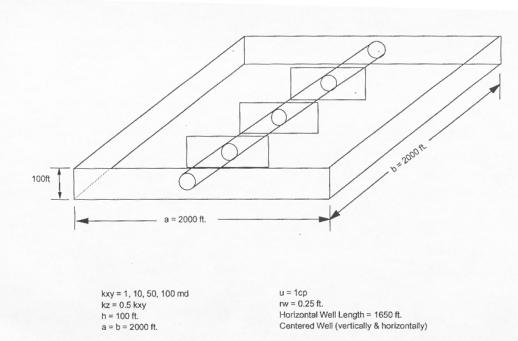
Figure 16. Schematic view of the layout for the fractured horizontal well tool.
Other assumptions and procedures include:
Ø single
phase, Darcy flow,
Ø fully
penetrating, infinite conductivity vertical fractures,
Ø finite
(closed) drainage area,
Ø The
injectivity Index is computed after pseudo-steady state flow has been reached, and,
Ø 1, 3, 5
and 7 (odd number) fractures are arranged in a symmetric pattern.
Sponsor Presentations
Paul van den Hoek provided case studies from
Oman, Thailand, Nigeria and Syria. The
first examples were from line drive waterflooding operations in Oman using
horizontals as the injectors. Figure 17
is a plot of sandface pressure versus rate.
Figure
17. Formation face pressure versus
injection rate (operations in Oman).
Chronologically grouped data are
indicated in Figure 17. Originally,
there was probably some matrix injection.
Subsequently, the flat behavior of the curve in Figure 17 suggested
fracturing (either induced or injection into natural fractures. The mobility in this reservoir is low, since
the in-situ oil viscosity is approximately 60 md. Some skin has developed due to water quality. This is shown by the higher than initial
injection pressure for the period of injection after a long shutdown (refer to
the labels on Figure 17). This could
also be due to some pressure buildup in the reservoir. To maintain matrix conditions, the capacity
of a 1-km well was only about 1200 BWPD, which is economically
unacceptable. One of the important observations made was the
low slope of the curves if friction is correctly represented.
Paul then presented a slide on a
NAM, showing similar behavior (Figure 18).
Figure 18. Formation
face pressure versus injection rate (NAM example), showing likely fracturing
behavior at a stress smaller than was originally assumed as well as flat or
slightly negative sloped curves – arising when friction is calculated
accurately.
The next example that Paul showed was from Thailand
(Figure 19) where there seems to be fractured injection from day one. Looking at the chronological variation in
behavior, trends move up and down but remain relatively parallel to each other.
Figure 19. Fractured
injector in Thailand.
The reservoir pressure was
likely impacting the fracturing pressure.
Jean-Louis Detienne asked if the water quality was unchanged. Paul indicated that it was constant (clean
aquifer water).
The next Shell field case was from Nigeria. This is an oil reservoir and is soft sands. The behavior shown in Figure 20 is very similar to behavior seen in the Elf 3 soft sands well. It is evident that there were numerous shut-ins and the II increased after shutdowns. There were probably backflow operations providing some sort of stimulation. John Shaw questioned whether the backflowing caused the well to sand up. Paul indicated that indeed the perforations were eventually covered up. After a CT clean out, it was found that the II was much lower than before. Marco Brignoli indicated that this did not surprise him and that the sand had been compacted. Marco indicated that after liquefaction you could see a substantial reduction in permeability. Bruce McIninch argued that viscous pills might have been another cause.
Some argument was made that this
was a situation that was taking fluid above fracturing pressure. Laurence Murray asked about screens and Paul
van den Hoek indicated that it was necessary to fracture the well for adequate
capacity.
Figure 20. Chronological
variation of the Injectivity Index and the bottomhole pressure for the Nigerian
well.
Figure 21. Variation of calculated sand frac pressure with injection rate for the Nigerian well, suggesting that some form of fracturing had probably occurred.
Paul next showed measured and simulator data for an injector in Syria. This is competent rock and the injection water is river water treated down to 10 mg/l. Simulations were done with varying solids loading and with varying temperature. Figure 22 is one match.
Figure 22. Variation of
injection rate with a superimposed rate profile used in various
Shell-proprietary simulations (Figure 23).
Figure 23 shows simulations for 10, 75, 95 and 110 mg/l and actual data. It can be seen that the injection pressure can move up or down by 1,000 psi depending on the solids loading. Recall that the water was filtered to 10 mg/l - at least at the surface.
Figure 23. Variation of
wellhead pressure with time in various Shell-proprietary simulations – TSS was
a variable.
It appears from the simulations that water quality can indeed be a significant controlling factor on pressure and there are substantial economic tradeoffs. In this case, the operator preference is not to buy new pumps to handle higher pressures but to clean the water.
For some time, Shell has been
developing a customized produced water fracturing simulator. It is desirable to forecast fracture and
pressure containment. The simulations
can be used as a tool for optimizing injector strategy.
Some checking of the PEA-23
relationship was carried out. Paul
emphasized the need for a SRT and that it is essential to calculate the correct
slope.
The model used calculates
conductivity based on a volume balance.
Paul concluded by expressing Shell’s future interests. These include:
- Comprehensive
analysis of Sponsor field data plus proper reporting of this
- Water
injection fracture monitoring (falloff, HIT,)
- Best
Practices for injectors in soft formations (completion, operation)
- Impact
of contaminant on injectivity for fracced injection (‘beyond PEA-23
relationship’)
- Fracture
growth/containment at material property boundaries (i.e., delamination,
containment even if there is not a strong stress contrast …).
Laurence Murray then presented
various examples. The first example
related to reduction
in injectivity due to water hammer effects. Unfiltered seawater (almost all < 4
microns) was being injected below fracturing pressure into three cased and
perforated zones. In this example
frequent shut-ins have been required and reverse circulation has been used for
cleanup. There were successive
reductions in this weak, relatively soft formation (E ~ 500,000 psi) due to
perforations being covered. When the
sand fill was cleaned out, the injectivity was reversed. There was gradual fillup that can be
characterized by a partial penetration skin.
The modulus is high enough that there actually has been some thermal
fracturing. Performance during injection
is tubing limited. In addition to
partial penetration there is also another skin component due to deviation
through the reservoir (since the deviation is small the associated negative
skin due to inclination is correspondingly small – see Earlougher, 1977, page
157). If you are careful, fillup can be
used to your advantage. If the rate of
fill up is not too rapid, progressive coverage may allow the well to
fracture. It was argued that you can
frac the sand away if you don’t come past the top of the perforations.
Laurence’s second example was
for cased and perforated platform wells.
All zones were covered (single zone) to avoid crossflow-related
problems. One well is at 75 to 80° and
the other discussed was vertical. One
of the concerns here was BaSO4 precipitation. There were substantial concentrations of
water-soluble organics. To manage this
phosphoric acid was used. Using the
PEA-23, for a permeability of 200 md ± there
was no real evidence of a substantial impact for the water quality being used
(from 10 to 20 or 25 ppm). Since
surface filters (cartridge) were blinding off, filtration was stopped and no
real performance difference was perceived.
The first well was pressuring up the reservoir. Perforations were added to the second well
and it was a well voidage completion.
Laurence argued that Well 1 was fraced and that the fracture closed down
with increasing stress levels due to poroelastic effects. It was emphasized that this can dramatically
impact reliable interpretation of Hall plots.
The Hall plot presumes constant kh.
If the height open to the fracture changes (part of the fracture
closes), response would be similar to an increase in skin and the plot would be
worthless.
There was some consideration to
back off on Well 2 and to try and clean up Well 1. The reservoir is weak (E ~ 100,000 to 200,000 psi), the net to
gross ratio is low, and the permeability is low (60 md). Almost all of the injection is at the
top. Originally this was a frac packed
produced and it appears that an injection induced fracture probably occur
adjacent to the fracpack, going into an unpropped fracture.
The next case study related to
falloff interpretation in a weak formation.
Both production and injection tests had been done. The completion was an openhole WWS. There were waxing problems associated with
cooldown in the wellbore and associated problems with the screens. The screens plugged during injection. What is required to match pressure transient
data for such a situation? It was
matched by using a damaged zone around the well. There
was a different size of damaged zone depending on whether you are injecting or
producing. Dale Walters
pointed out the compaction zone ahead of a fracture.
Laurence also showed a BP PWRI
Best Practices web-based presentation.
One of the unique features was the ability to viewed threaded comments.
At this point there was a
discussion of skins and how to use them in PWRI situations. For example:
- Filter cake ahs no mechanical strength but
causes a pressure drop. Presence
of a filter cake can help fracturing.
The fracture grows through the skin; the rate goes up and
eventually performance is tubing limited.
Partial penetration may need to be considered because the cake
and/or fracture may develop and evolve (or devolve) preferentially.
- It may be desirable to complete the well as a
partial penetration (actually this is more accurately called a partial
completion) so that you can initiate a fracture and you at least know
where it starts.
- Another skin scenario is internal cake where
the differential pressure can inhibit getting pressure into the formation.
The obvious related topic is
“How should you complete multi-zone wells?”
There was some sentiment that flow control may be a prerequisite.
There was discussion about
fracture containment. Laurence
indicated that BP has seen it in some cases (particularly Prudhoe Bay) where
there is not substantial stress contrast and it could be related to
conduction/convection. Out-of-zone
fracturing may ensue.
In some wells where sidetracks
have been drilled above the main bore; they have gone into areas that have
already been cooled by conduction.
Mechanical control may be required.
Laurence will provide an example of this.
Another area of discussion was
for soft rock, with injection above fracturing pressure – What role does water
quality play? For example:
- What are the criteria for screen plugging?
- Can hot spots develop?
- Hot spots may preferentially develop when you
fracture because of high concentrated velocities.
- What about hot spots in ESSs?
Bruce McIninch recounted their
experience with screen testing for West Brae.
They found two things. One was
that friction was not significant and two the testing was beneficial because it
allowed them to specify a redesign to the manufacturer.
John Shaw described two field
trials that are being run by Statoil.
The first is the Statfjord test.
John showed a Hall plot and discussed several monitoring issues. Protocols on one well have included running
seawater at 30°C, followed by a 50/50 seawater/produced water at approximately
55°C. Injection is into the Upper Brent
(permeability is approximately 670 md).
There has been a drop in reservoir pressure and some rate increases during
the pilot. The Hall plot showed a
significant increase in injectivity with produced water due to viscosity
effects. They are now switching to 100%
produced water (75°C). Step rate testing
has shown a thermal stress affect of 1 bar/°C. The injected produced water is low in oil
but high in solids (up to 250 mg/l).
The next pilot was Heidrun. This is soft, heterogeneous and there is a
good amount of clay. The well is cased
and perforated in five zones over 45 m, with permeability ranging from 150 to
350 md. They have injected seawater
(30°C) since November 1999 and the rate has been dropped from 3000 to 2000 m3/day. Subsequently they switched to produced water
at 60°C. The water quality is extremely
poor. If you evaluate the Hall plot,
for the initial seawater part, you see two distinct slopes. Another seawater injection seemed to show a
second breakdown. A produced water test
was then done. It seems as if a
fracture has been established and is taking fluid. There is not classical matrix behavior (the rate stays up).
Idar Svorstol then presented on
Norsk Hydro's work on Snorre. 43 wells
have been developed so far and a new platform will be installed in the North -
with 16 producers and 10 injectors.
Production will start in August 2001.
These wells have intelligent completions. This entails sliding sleeves and bottomhole gages. The program also includes cuttings
reinjection.
Current Snorre capacity is
approximately 40,000 sm3/day.
Some of the issues on Snorre are environmental - the deoxygenation can't
handle any more seawater. In addition,
Snorre involves high and low permeability zones and problems might be
anticipated for lower water quality situations.
Jean-Louis Detienne indicated
that he will be getting two or three more field cases but they will not be
available soon. Jean-Louis expressed
his opinion on the requirements for the overall PWRI project. He indicated that it is necessary to process
all of the available data and to get the tools into the hands of the Sponsors
and to give feedback on the Toolbox.
AGIP provided new data to the Contractors
for an aquifer injection situation (it is a good case study since one well is
fractured and one is probably taking fluid under matrix conditions).
Laurence Murray provided another
example - relating to openhole gravel packed wells. Underreaming before gravel packing was designed so that there
would be enough pack for fines to accumulate in. Water hammer cleanup was also discussed.
Trond Jensen discussed Ekofisk
seawater injection that has been carried out on the flank for 12 years. Pressure has increased and injectivity has
gone down. This is for clean,
deoxygenated seawater. It is batch
treated with biocide, ultraviolet exposure and filtration down to 2 microns. The Hall plot shows a change in slope. Trond is uncertain as to whether the change
is due to real skin development or to a change in reservoir pressure, although
he favors the former.
There was further discussion of
souring evaluations on pilots and whether backflowing would provide substantive
information. John Shaw felt that it was
possible but he was skeptical.
Ahmed Abou-Sayed presented
several options for development of an economic module for PWRI. These were:
Option 1. A comprehensive model, based on the
platform and database provided by Paul van den Hoek.
Option 2. A spreadsheet that is a stripped down
version of the Shell model, with comparative costs.
Option 3. A spreadsheet with categories but no
comparative cost information.
Option 4. A checklist based on the flowchart
presented by Advantek at the December quarterly meeting.
Option 5. Abandon the Task.
Sponsors expressed their
preference by vote, as indicated below.
- Marco
Brignoli indicated that AGIP's preference would be not to have an in-depth
tool. He opted for Option 3.
- Jean-Louis
Detienne indicated that he was interested in the flow chart structure that
Advantek had presented at the December Meeting. He indicated a preference for something simple (Option 3).
- Idar
Svorstol indicated that while he did not have a strong opinion on this
particular issue, his preference would be something that is not too
detailed and would provide a rough idea of the economics. His vote was for Option 3.
- Henrik
Ohrt selected Option 4 in order to safeguard (be sure that previous
efforts are available) what has already been done. He is just interested in a
checklist. He would accept Option
5 but would vote at this stage for Option 4.
- John
Shaw voted for Option 5, but "could live with Option 3 if
necessary."
- Laurence
Murray opted for Option 4, to have a methodology for just seeing if all of
the bases are covered.
- Paul
van den Hoek strongly supported Option 1 and would not go down below
Option 2. "Anything else is a
waste of time."
- Trond
Jensen indicated his interest in comparative costs but he believes
accomplishing this is not practical.
His vote was for Option 4 and Option 3, if absolutely necessary.
- Bruce
McIninch only wanted a checklist (Option 4).
Options 3 and 4 had three votes each. The decision was made to opt for Option 4.
Based on a suggestion from
Henrik Ohrt on the previous day, John McLennan tried to outline some of the
accomplishments and future requirements for the JIP. This presentation is available.
This presentation can be summarized as follows.
Five Key Findings
- If reservoir pressure is not reliably
considered and if formation face pressure is not reliably represented, any
sort of diagnostic or predictive methods are potentially in significant
error. This is a trivial but
essential concept. Tools are
available for representing these features in fundamental, continuous
injection monitoring evaluations.
Consequences
of not reliably knowing formation pressure and formation face pressure include
inability to plan when treatments should be carried out and to recognize
fundamental degradation in injectivity, misinterpretation of pressure transient
data, inadequate/inappropriate support, incorrect decisions on the type of
intervention that is required, if any, etc.
Many reservoirs are being fractured and it has not been appreciated -
except by specialists - sweep considerations, etc.
- The PEA-23 concepts can be extended/modified
to quantify discrete events representing extension/growth of
fractures/discontinuities even in unconsolidated formations. More quantification is required in the
next three months using available data.
Data are available for calibrating available models.
Consequences: Design tools and “vision,” stimulation
planning and optimization of investment for maintaining injectivity
- There can be a point of diminishing or no
return in stimulation beyond which further “conventional” stimulation will
provide progressively less effective results.
Consequences: Methods are being developed to represent
this during the current phase of the project using back-analysis of available
injection history. Stimulation types
can be refined – using this and the concepts in Key Finding 2.
- Near-wellbore skin, particularly completion
skin is an under-appreciated feature in comprehending injection
programs.
Consequences:
It can be huge in soft formations and misrepresent required
stimulation/intervention. It can
possibly be manipulated to achieve improved conformance. It may entail significant perforation fillup
in soft formations and its magnitude and impact can vary depending on whether
injection is above or below fracture opening/reopening pressure.
- The complexity of fracture growth in
consolidated and in soft formations is such that planar, single fracture,
constant height or ellipsoidal fracture models may be inadequate in many
cases. Consider cases where they will
be inadequate – in layered reservoirs with significant stress or
permeability contrast where fracture or matrix fingering dominates, in
weakly consolidated reservoirs, in reservoirs where there are multiple
fractures that are created by pressure cycling (does not even need to be
batch injection), in untuned (the injection program has not been
fine-tuned for optimum performance in a specific reservoir based on
historical response) reservoirs with injection just below fracture
extension pressures, in naturally fractured reservoirs treated at low (or
possibly cycled) injection rates.
Consequences: Cautious or selective use of LEFM (linear
elastic fracture mechanics) is essential.
The wellbore and the completion must be reliably represented. Disposal domain concepts may be a
pre-requisite. Vertical fracture growth
must be represented.
Five Key Achievements (not
prioritized)
- Availability
of Data
·
Acquisition of data!
·
Archiving of data!
·
Using data!
·
Although it has been slow, the development of the database
and the interpretation of the data are approaching the point where information
is being more effectively archived and processed.
·
Before the end of this phase, more needs to be
completed. Much of the intellectual
maturation in this project has come about from looking at trends in and features
of available data by a diverse group.
- Development/Organization
and Ultimate Deployment of Analytical Tools
Examples
of tools developed include:
·
Completions Worksheet
·
PWRAD
·
Multilateral/Multifracture Models
·
Stimulation Selection Tool
·
Thermal and Poroelastic Stress Tool
·
Data Management Capabilities (BHP, plotting …)
·
Others
- Knowledge
Management/Best Practices/Assurance
Consolidation
of available findings is being accomplished by incorporation into
guidelines. Key issues are being prioritized
as Best Practices. These include
supplementary information for design and outline, where possible, procedural
limitations. Methodology has been
developed for logically archiving and providing accessibility.
- Workshops,
Exposure and Interaction
While it
is somewhat more philosophical, Workshops and Quarterly meetings have
facilitated:
·
Presentation of case studies
·
Shared experience and platform for communication
·
Constructive criticism by a diverse audience
·
Exposure to experience from other disciplines
- Recognition
of Concepts, Methods, Limitations and Future Requirements
Examples
include:
·
Definition of inadequacies in current testing
methodologies (e.g. SRT, falloff in layered formations)
·
Definition of limitations in modeling methodologies
·
Consolidation and outlining of various options for
completions and stimulation (e.g., conformance methods, procedures for bringing
horizontals on-line, the future role of intelligent completions, ESSs, fiber
optics, indirect appreciation of the economics of surface treatment versus
stimulation, possible occurrence of a compacted zone …)
Main Recommendations
Recommendations were presented
as to what some of the future or ongoing work might be. This is a Contractor's perspective and does
not necessarily reflect the position of the Sponsors.
- Maintenance
and Updating of Tools, Best Practices, Database
This
would seem desirable as data has driven much of the project (database). Even through the duration of the project,
opinions and conceptual appreciation have evolved. Tools developed in the Project were not necessarily envisioned at
the outset. Additional, high quality
data are anticipated from upcoming or ongoing pilots and field programs. This would also help to maintain
communication among a diverse group
- Case
Studies
·
Each Sponsor will be requested to continue to provide
field data.
·
These data may in fact be superior to some of the
historical data that have been provided because of improvements in
instrumentation, acquisition, and experience/knowledge.
·
Information will be incorporated into the database system
and evaluated with specific intent of testing/improving tools that have been
developed, conceiving/recommending/developing of new tools, concepts, learnings
and identifying physical behavior.
- Workshops
·
Two workshops were suggested – one after six months and
one after nine months?
·
Each of these would be designed to look at new
technologies and at new and recent developments or events.
·
It was recommended that the first Workshop cover horizontal
injectors and that the second Workshop would incorporate important aspects from
all of the Tasks in the first phase of the JIP.
·
There would be quarterly meetings, two of which would
coincide with the Workshops.
- Miscellaneous
·
Accounting /Contractual
·
Management: Recording and posting of minutes,
coordination, interaction with Sponsors on performance issues and interaction
with Contractors to improve delivery, etc.
·
Travel: Will need to be preauthorized for four travel
sessions (quarterly).
- New
Tool Development
The
following four areas of Tool development are described adequately in the presentation.
·
Diagnostic Methods (e.g. PTA methods)
·
Predictive Model (PWSIM)
·
Completions Skin Tool
Thursday March 29, 2001
Sponsors met and reviewed the requirements for proceeding forward to complete the existing Project and evaluate mechanisms for developing additional deliverables with the funding remaining in the Project.
Laurence Murray summarized the
results of the Sponsors meeting.
Laurence’s remarks are summarized below.
Project Administration:
A firm proposal is
required. A new contract is required
that gives a flexibility to the work beyond June 30th. Contracts stop at the end of March. There is no mechanism for payment. GTI have given a proposal as an interim
solution - at least until the end of June.
This has been rejected because of a monthly cost of approximately
$10,000. The Sponsors are amenable to a
small fee to GTI to transfer the contract to another party.
Mentors:
To facilitate proper completion
of the initial phases of the project, a group of Mentors was agreed upon. These are:
|
Task |
Mentor(s) |
|
Monitoring
and Prediction |
Laurence
Murray and Mark H. |
|
Matrix
Injection |
Paul
van den Hoek and Henrik Ohrt |
|
Soft
Formations |
Jean-Louis
Detienne |
|
Stimulation
and Mitigation |
Henrik
Ohrt and Paul van den Hoek |
|
Layered
Formations |
Trond
Jensen and Idar Svorstol |
|
Horizontals |
|
|
Database |
All
Sponsors |
|
Surface
Systems |
John
Shaw |
|
Validation |
John
McLennan |
|
Best
Practices |
All
Sponsors |
|
Web
Site |
All
Sponsors |
Requirements for Completion:
For all Tasks there are some basic requirements. Some specific requirements were required for
individual Tasks. For example”
Ø
For all Tasks: An essential requirement is final reports,
including descriptions of relevant tools with worked examples.
Ø
For the Database, a User Guide is required. The database needs to operate as a
standalone PC version and there needs to be an equivalent web-based
version. This is in effect and Brian
Odette will continue to see that it is implemented.
Ø
Best Practices: Some additions need to include an overview
of the JIP and a summary of the achievements.
It must also contain guidelines and relevant reports and documents.
Ø
Website: As with the database, there needs to be a web
version and a CD version.
Ø
In the minutes, footnotes or descriptors need be added to
the viewgraphs and slides.
Ø
For the Validation Task, it is necessary to incorporate
field testing results where they are available. An Opportunities List needs to be developed and circulated.
Ø
Surface Systems: Final reporting is required, as is a
Users’ Guide. The Surface Systems
component of the project needs to be web- and CD-based. The final report needs to cover some of the
technical issues. What are the key
things that you need to be looking out for?
Some sort of guide for using.
Ø
Validation: As field data comes in, evaluate these data
and see what is derived and make the results known. There needs to be feedback on the validity of tools, models, etc.
Ø
Toolbox: The requirements include a finished working
version, including a Users’ Guide that incorporates a technical manual for the
tools.
Ø
Best Practices: Incorporate a JIP Overview, achievements,
guidelines and documents.
Ø
Website – can also run off a CD. Also, where data have been interpreted, it is important to
clarify the analytical methodology.
Future Work:
A firm proposal is
required. There are some minimum
requirements, as listed below that need to be accomplished and/or continued before the end of June.
- Website, toolbox, database guidelines –
working finished version by the end of June.
- Web site maintenance
- Database maintenance
Using the oversubscribed funds, the Sponsors will consider
proposals for work from July 1, 2001 to
June 30, 2002. Some of the
components need to be:
- Database
and Website Maintenance – to maintain the current
status and to add information to it.
- Upgrade
of Toolbox, Best Practices and Existing Guidelines It
is important for the Task Mentors to actually study and test to identify
bugs, errors, omissions …
Upgrading would entail increasing the functionality or implementing
new tool(s). An example of
upgrading the Guidelines would be to indicate if somebody has carried out
a new technique
and has new experience.
Consolidation into existing Guidelines would be required.
Beyond these basic Tasks for continuation,
there is motivation to carry out certain additional or new
Tasks/Developments. These could
include:
- Pressure Transient
Analysis: Starting from the Monitoring Workshop in Denver, it
was evident that improved pressure transient analysis methods are required
for single and multiple layer scenarios.
- Predictive Model:
During the first phase of the Project, comprehensive predictive model
development was discouraged in order to focus on evaluation of data. There is some feeling that a more
comprehensive tool could be proposed.
Laurence Murray indicated that he supports some sort of standalone
tool that everyone (including their partners) can use, possibly a module
that can be put into a commercial simulator. There was discussion relating the costs and scope of such a
model. For example, Paul can den
Hoek felt that models were going to cost hundreds of thousands of dollars
to couple to reservoir simulators.
In any submitted proposal, it was stressed that it was important to
identify the functionality of the proposed model (e.g. local grid
refinement?, wellbore management functions?, …).
- Completions
Skin Tool: One of the issues that has been strongly identified during the
course of the Project has been the importance of specific completion
characteristics. One possible
component for future work was identified as a tool for characterizing
completion behavior, as has been done to a certain extent for
perforations.
During the in-camera session, the Sponsors prepared a prioritized list of desirable components for future work. This was not passed onto to the Sponsors. Laurence Murray indicated that this would be circulated to Sponsors (by the middle of April) so that a Sponsor position could be developed on how to usefully spend the remaining money.
Date for the Next Meeting:
The meeting was scheduled for
the last week of June, in Houston. The
dates would be Monday, June 25 through Thursday, June 28. All participants are requested to plan on
attending the complete session. A
hosting organization will need to be identified.
Prior to the meeting, it is
desirable for Sponsors to review the current Project and, in particular, for
Task Mentors to dig into some of the details.
Any Sponsor review should be given back to the Contractors by the first
of June.