Analysis of Stimulation of Elf3 Water Injectors
Reservoir
Data from two injectors were analyzed. The reservoir is an unconsolidated sandstone reservoir.
Well W1. Well W1 has a permeability of approximately 1700 mD and a porosity of 26%. The initial reservoir pressure was estimated to be 176 bar or 2550 psi. Reservoir pressure during injection was not measured and a constant reservoir pressure was assumed in the analysis. The reservoir temperature is 70 deg C or 160 deg F. The best estimates on the initial minimum horizontal stress is 0.14 to 0.16 bar/m or 0.62 to 0.71 psi/ft. The perforation intervals have a true vertical depth of 1548 - 1566 meter and 1597 - 1615 meter or 5079 - 5138 feet and 5240 - 5299 feet. Initial fall-off test of October 1991 indicated an initial skin of 22.5. Fall-off test of June 1994 gave a skin of 460.
Well W2. Well W2 has a permeability of approximately 4000 mD and a porosity of 24%. The initial reservoir pressure was estimated to be 140 bar or 2030 psi. Reservoir pressure during injection appears to be constant from fall-off tests. The best estimates on the initial minimum horizontal stress is 0.14 to 0.16 bar/m or 0.62 to 0.71 psi/ft. The perforation intervals have a true vertical depth of 1262 - 1274 meter and 1622 - 1639 meter or 4140 - 4173 feet and 5322 - 5377 feet. The reservoir has a true vertical depth of 1256 m - 1284 m or 4120 ft - 4210 ft. Initial fall-off test of October 1996 indicated a skin of 500 and the skin was reduced to 180 after acid stimulation.
Water Source and Quality
Only produced water was injected into both wells since start-up of the wells. Temperature at the surface was 67 deg C or 163 deg F, almost the same as the reservoir temperature. Viscosity of the water at the surface is 0.45 cP. The produced water was filtered to particle sizes of less than 50 mm. There was not water quality history data - the estimated total suspended solid concentration was 3 mg/liter and the oil-in-water concentration was 200 ppm.
Stimulations
Numerous acid simulations were conducted during the six-year injection history for well W1 and the four-year injection history for well W2, with both 15% HCl acid of different volumes and inhibited river water. Table 1 shows the stimulation fluid and volume for each of the stimulation performed on well W1 and Table 2 lists the stimulation fluid and volume for well W2. As can be seen from these tables, there is less variation in acid volumes for well W2 stimulations than for well W1 stimulations.
Table 1. Stimulation
Fluid and Volume for Well W1
|
Stimulation |
Stimulation |
Treatment |
Treatment |
|
1 |
15% HCL |
5 |
31.5 |
|
2 |
15% HCL |
5 |
31.5 |
|
3 |
15% HCL |
4 |
25.2 |
|
5 |
15% HCL |
4 |
25.2 |
|
6 |
15% HCL |
2 |
12.6 |
|
7 |
15% HCL |
0.8 |
5.0 |
|
8 |
15% HCL |
2 |
15.6 |
|
9 |
Inhibited Water |
|
|
|
10 |
River Water |
|
|
|
11 |
15% HCL |
2 |
12.6 |
|
12 |
15% HCL |
2 |
12.6 |
|
13 |
15% HCL |
? |
|
|
14 |
Inhibited Water |
|
|
|
15 |
15% HCL |
0.8 |
5.0 |
|
16 |
15% HCL |
4 |
25.2 |
|
17 |
15% HCL |
4 |
25.2 |
|
18 |
15% HCL |
5 |
31.5 |
|
19 |
15% HCL |
2 |
12.6 |
|
20 |
15% HCL |
4 |
25.2 |
Table 2. Stimulation
Fluid and Volume for Well W2
|
Stimulation |
Stimulation |
Treatment |
Treatment |
|
1 |
15% HCL |
1.6 |
10.1 |
|
2 |
15% HCL |
1.6 |
10.1 |
|
3 |
15% HCL |
1.6 |
10.1 |
|
4 |
15% HCL |
1.6 |
10.1 |
|
5 |
15% HCL |
1.6 |
10.1 |
|
6 |
15% HCL /w I.W. |
0.8 |
5.0 |
|
7 |
15% HCL /w I.W |
0.8 |
5.0 |
|
8 |
River Water |
30 |
188.7 |
|
9 |
15% HCL |
1.6 |
10.1 |
|
10 |
Inhibited Water (I.W.) |
25 |
157.3 |
Matrix Injection or Injection Under Fracturing
Figure 1 and Figure 2 show the bottom hole pressure versus injection rate for well 1 and for well 2, respectively. The reservoir pressures for the two injections were estimated initially to be 2550 psi and 2030 psi, respectively. It may be difficult to conclude whether the injections were under matrix conditions or under fracturing conditions. Figure 1 shows that the bottom hole pressure slightly decreased as injection rate increased, indicating injection under fracturing condition. However, this decrease in bottom hole pressure may be due to frequent stimulations as shown in Figure 3. Considering the large skin (460) from fall-off test some three years after start-up, it would be difficult to conclude this injector was under fracturing conditions - injectors under fracturing conditions would produce negative or low skin.
Figure 2 shows that this injector appears to be under matrix injection. This is consistent with the large skin (500) from fall-off test on this injector.
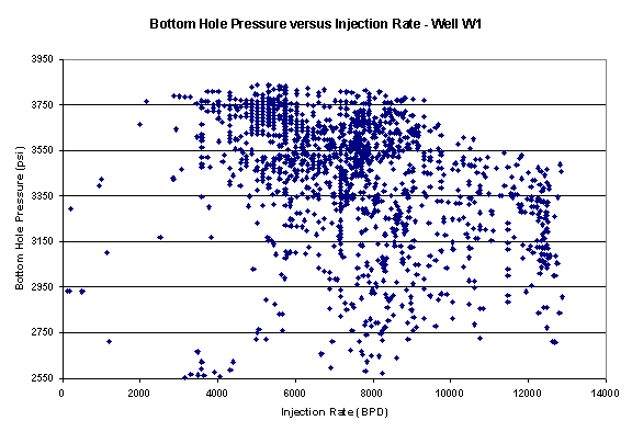
Figure 1. Bottom hole pressure versus injection rate. It appears that the bottom hole pressure decreased slightly as injection rate increased. This could be due to frequent stimulations, see Figure 3 in the following. Large skin factor (460) from fall-off test would indicate matrix injection.
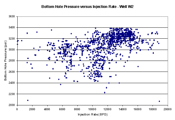
Figure 2. Bottom hole pressure versus injection rate. From this figure and considering the large skin (500) from fall-off test, one may conclude that the injector was under matrix injection.
The Injection History
Figure 3 shows the Hall plot for well 1, with stimulations indicated by the vertical lines. Figure 4 shows the Hall plot for injector 2, again with stimulations indicated by the vertical lines. Figure 5 through Figure 7 show various stages of processing the available information for well 1, with rationale and observations included in the figure captions; the wellhead pressure and wellhead injection pressure and injection rate history. It should be noted that constant reservoir pressure of 2550 psi was used in calculating the injectivity index as shown in Figure 7. Figure 8 through Figure 10 show various stages of processing the available information for well 2, again with rationale and observations included in the figure captions. the wellhead pressure and wellhead injection pressure and injection rate history. A constant reservoir pressure of 2030 psi was used in Figure 10 for the injectivity index calculation.

Figure 3. Ideal Hall plot (assuming no further damage after stimulation), improvement ration (ratio of injectivity index after stimulation to before simulation), overlay on top of Hall Plot. As can be seen, there is a clear benefit of acid stimulation.

Figure 4. Hall plot and improvement ratio. As can be seen, there is a clear benefit of acid stimulation. It also shows that benefit of some simulations is sustainable after the simulation for quite sometime.
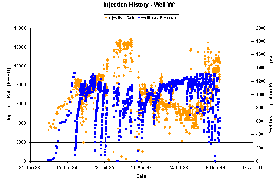
Figure 5. Wellhead injection pressure and injection rate history plot for well W1.
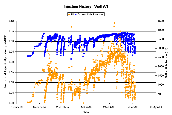
Figure 6. Bottom hole pressure and reciprocal injectivity index history plot for well W1.

Figure 7. Reciprocal injectivity index versus cumulative injected water volume. Also plotted in this figure are the indicators of stimulations (vertical line) and the base-line value (horizontal line).
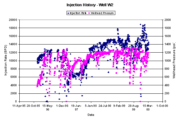
Figure 8. Wellhead injection pressure and injection rate history plot for well W2.
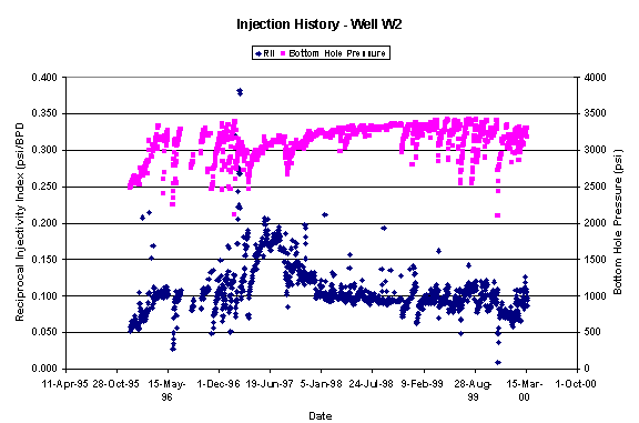
Figure 9. Bottom hole pressure and reciprocal injectivity index history plot for well W2.
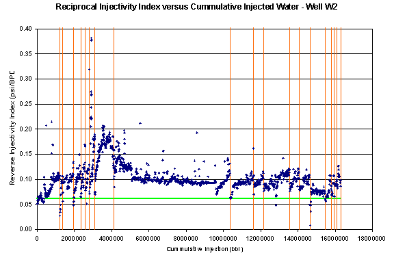
Figure 10. Reciprocal injectivity index versus cumulative injected water volume. Also plotted in this figure are the indicators of stimulations (vertical line) and the base-line value (horizontal line).
Stimulation Results and Correlation Development
Two parameters are defined here in presenting the stimulation results. One is improvement ratio, which is defined here as the ratio of the injectivity index after the stimulation to the injectivity index before the stimulation. It is a measure of initial stimulation performance. The injectivity indexes are determined from the intersection values. Another parameter normalized reciprocal injectivity index, DRII, is defined by the following equation:
![]()
where the RII is the intersection value (on the simulation line) of reciprocal injectivity index and RIIbaseline is the lowest 30-day moving average RII value. The baseline value is 0.038 for well 1 and 0.061 for well 2.
For each stimulation, the developed Toolbox was used to analyze the data. First, the reciprocal injectivity index was plotted against the accumulative injection volume. Then, linear curve-fitting was applied to both the pre-stimulation portion and the after-stimulation portion of the data. Reciprocal injectivity indexes (and thus injectivity indexes) at stimulation, both before and after stimulation, can be obtained from the interception values of the curve fits. The slopes or injectivity index decline rates, both before and after stimulation are obtained from the slopes of the curve fits. This analysis procedure is shown schematically in Figure 11. Results from the stimulations for the two wells can then plotted and analyzed to develop necessary correlations for predicting after-stimulation performance from pre-stimulation information.
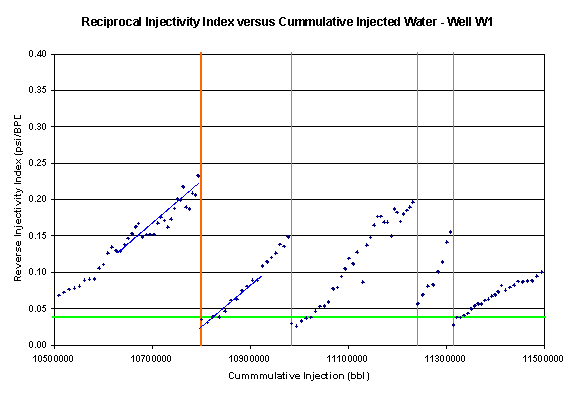
Figure 11. Schematic of linear curve fit before and after stimulation.
Correlations of Improvement Ratio and Pre-Stimulation Information
The objective here is to predict initial after-stimulation performance such as injectivity index immediately after stimulation or improvement ratio, from pre-stimulation information such as the injectivity index, or injectivity decline rate.
Figure 12 shows after-stimulation injectivity index versus pre-stimulation injectivity index for both wells. As can be seen, there is a better correlation between the initial after-stimulation performance and the pre-stimulation injectivity index for well 2 than for well 1. This is because that the stimulations on well 2 are more consistent in terms of acid volumes than for well 1. Figure 13 shows the acid volume effect on after-stimulation performance. As expected, more acid volume yields better initial after-stimulation performance. Figure 14 is a cross-plot of after-stimulation injectivity versus pre-stimulation injectivity decline rate. It shows that there does not appear to have correlation between the after-stimulation injectivity index and pre-stimulation injectivity decline rate. Figure 15 shows the improvement ratio (the ratio of after-stimulation injectivity index to pre-stimulation injectivity index at the time of stimulation) versus normalized pre-stimulation reciprocal injectivity index, which is defined as difference between the pre-stimulation reciprocal injectivity index and the baseline value of reciprocal injectivity index, divided by the baseline value of reciprocal injectivity index.

Figure 12. Injectivity index before and after each simulation for both well W1 and W2. As can be seen from the plot, although there is a good correlation of stimulation results on well W2, there is a quite large scatter from the stimulation results on well W1. This may be due to the fact that this well was stimulated with different treating fluids and different volumes, which is shown in the next figure. Stimulations on well W2 were relatively consistent, in terms of acid volume per stimulation (from 0.8 to 1.6 m3 or 5 to 10 barrels).
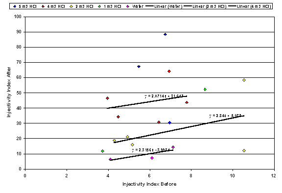
Figure 13. Cross plot of after-stimulation injectivity index and injectivity index before stimulations for well W1 with different stimulation fluids (15% HCl and inhibited river water) and volumes. As expected, more acid volume gives larger injectivity index after stimulations. Stimulations from inhibited river water gave the least improvement.
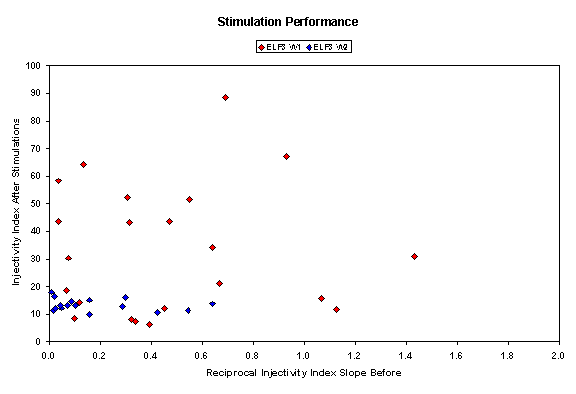
Figure 14. Cross plot of improvement ratio and reciprocal injectivity index increase per 1 million barrel of injected water before stimulations. As can be seen, it does not appears to have a strong correlation between the injectivity index after stimulation with reciprocal injectivity index slope before stimulation.
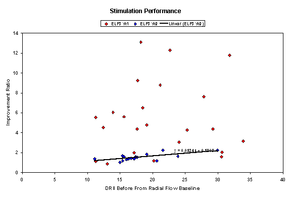
Figure 15. Cross plot of improvement ratio and DRII, which is defined as the difference of the reciprocal injectivity index from its base-line value, normalized by its base-line value. The base-line value is the value from radial flow. Different acid volumes were used in the stimulations for well W1 and there is quite large scatter of results, as seen in the plot. Stimulation results from well W2 show a much smaller scatter. This may be because stimulations on well W2 were done with relatively consistent acid volume, varying from 0.8 to 1.6 m3 or 5 to 10 barrels.
Correlations of After-Stimulation Slope and Pre-Stimulation Information
Slope of reciprocal injectivity index is defined as reciprocal injectivity index increase per 1 million barrels of injected water. After-stimulation (before-stimulation) slope is obtained from the linear-fit of reciprocal injectivity index after simulation (before stimulation) versus total injected water volume. After-stimulation slope measures how fast of injectivity decline after simulation - the slower the decline or the smaller the slope, the better.
The objective here is to predict how long the after-stimulation performance will last, in other words, to predict after-stimulation injectivity index immediately after stimulation decline rate from pre-stimulation information such as the injectivity index, or injectivity decline rate.
Figure 16 shows the after-stimulation slope versus pre-stimulation slope for both injectors. Figure 17 shows the after-stimulation slope versus pre-stimulation sloe for well 1 with different acid volumes. As can be seen from these two figures, there is a correlation between the after-stimulation slope and the pre-stimulation slope. In other words, one may estimate after-stimulation injectivity decline rate from pre-stimulation injectivity decline rate. Also can be seen is that stimulations with larger acid volumes yield smaller slope. Previously, it concludes that larger acid volume yields better initial after-stimulation performance. Figure 17 shows that this better initial after-stimulation performance with larger acid volume also lasts longer.
Figure 18 shows the after-stimulation slope versus pre-stimulation reciprocal injectivity index for both wells. Figure 19 shows the after-stimulation slope versus normalized pre-stimulation reciprocal injectivity index. Strong correlation is obtained between the after-stimulation slope and pre-stimulation or normalized reciprocal injectivity index. One can also use these correlations to predict after-stimulation injectivity decline rate from pre-stimulation performance.

Figure 16. Cross plot of reciprocal injectivity index slope per 1 million barrels of injected water after the stimulation versus the slope before the stimulation. It appears there is a reasonable correlation between the slope before stimulation and the slope after stimulation.
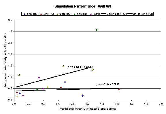
Figure 17. Cross plot of reciprocal injectivity index slope per 1 million barrels of injected water after the stimulation versus the slope before the stimulation. This is a plot for Well W1 only with different stimulation volumes.
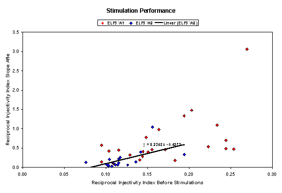
Figure 18. Cross plot of reciprocal injectivity index slope per 1 million barrels of injected water after the stimulation versus the reciprocal injectivity index before the stimulation. As can be seen, there exists a reasonable correlation between slope after simulation and the reciprocal injectivity index before the stimulation. The correlation may be used to estimate the slope after the stimulation, that is, how fast the improved injectivity will decrease, from the before-stimulation information.
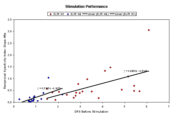
Figure 19. Cross plot of reciprocal injectivity index slope per 1 million barrels of injected water after the stimulation versus DRII before stimulation. Again, good correlations were obtained between slope after simulation and the normalized reciprocal injectivity index DRII before the stimulation. The correlations can again be used to estimate the slope after the stimulation, that is, how fast the improved injectivity will decrease, from the before-stimulation information.
Conclusions and Recommendations
1. From the bottom hole pressure versus injection rate plots and considering the large skin (460 for well 1 and 500 for well 2) from fall-off tests, one may conclude that the injectors were under matrix injection conditions.
2. Correlation was developed to estimate initial after-stimulation injectivity index or improvement ratio from pre-stimulation injectivity index or from the normalized pre-stimulation reciprocal injectivity index.
3. As expected, more acid volume yields better larger stimulation improvement. Correlations were developed for stimulation improvement estimates.
4. It concluded that there were no correlation between initial after-stimulation injectivity index and the pre-stimulation injectivity decline rate.
5. Correlation was developed between after-stimulation injectivity decline rate from pre-stimulation injectivity decline rate.
6. Correlation was also developed between after-stimulation injectivity decline rate from pre-stimulation reciprocal injectivity index or normalized pre-stimulation reciprocal injectivity index.
7. These correlations can be used to predict after-stimulation injectivity decline rate from pre-stimulation injectivity information.
8. Larger acid volume yields better initial stimulation improvement. More importantly, the initial better stimulation performance also lasts longer.
9. The developed correlations can predict future injectivity performance from pre-stimulation information. Based on the correlations and estimated produced water volume, one can estimate whether the extra produced water can be handled by the existing injectors through stimulation or new injectors are necessary. If new injectors are necessary, one may estimate when and how many, based on the correlations.
10. From the correlations, one can estimated after stimulation performance. Based on oil produced from the extra water injected, one can predict pay-back time for the stimulation cost during stimulation design phase.
11. Stimulation using more acid showed clear benefits. Correlations have been developed to study acid volume effects. These relations can be used to perform "what-if" studies in PWRI design and to estimate the pay-back times for the extra cost associated with more acid stimulation.