Field Elf 2 Well 1

The Reservoir

This is a carbonate reservoir with a permeability characteristically varying between 0.5 and 5 md and a porosity of 20%. The initial minimum horizontal stress was estimated to be 500 to 600 bars or 7250 - 8700 psi at the injection interval. The reservoir is at 2865 m TVD or 9400 ft TVD. The initial reservoir pressure was estimated to be 260 bars or 3770 psi. The reservoir pressure was decreasing during injection (see Figure 1). The reservoir temperature was 98^oC or 200^oF.

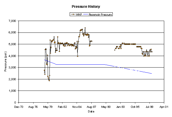
Figure 1. Reservoir pressure and wellhead pressure history. There is portion of missing data in the wellhead pressure.

The Water Source and Quality

For the first 4200 days, the injected water was from an aquifer (AW), with very small portions of produced water. From day 4200 to day 7000, the injected water was a mixture of produced water (PW) and aquifer water. After day 7000, the injected fluid was 100% produced water. Figure 2 shows the percentages of aquifer water and produced water during the course of injection for this well. The water temperature at the surface was 20^oC or 70^oF for aquifer water injection, between 20^oC and 50^oC (70^oF and 120^oF) for AW/PW injection and 50^oC or 120^oF for PW injection.

The water was filtered to 10 mm. Figure 3 shows the total suspended solids and the oil-in-water concentration.

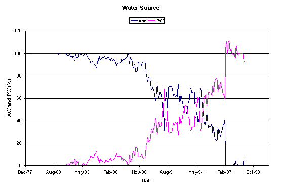
Figure 2. Water source history plot during the course of injection. As can be seen, in the early stages of injection the injected water was mostly aquifer water. Later, this was followed by a mixture of aquifer water and produced water and finally close to 100% produced water.

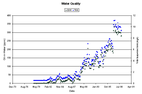
Figure 3. Oil-in-water and total suspended solid concentrations as a function of time. As can be seen, initially when aquifer water was injected, there is no oil in the water and the total suspended solid was very low. As expected, the water quality became worse and worse when the fraction of produced water was increased.

The Injection History

Figure 4 shows the wellhead injection pressure and injection rate history. Figures 5 through 8 show various stages of processing the available information, with rationale and observations included in the figure captions.

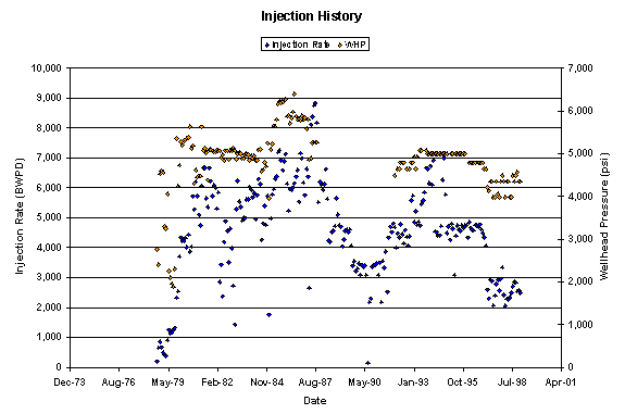
Figure 4. Wellhead injection pressure and injection rate history plot. As can be seen, there is a portion of missing data in wellhead pressure.

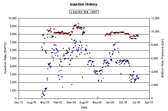
Figure 5. Bottomhole pressure and injection rate history plot. Each data point represents one month.

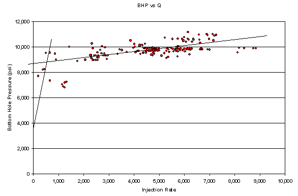
Figure 6. Bottomhole pressure versus injection rate plot – a step-rate “type” plot. It should be noted that each data point may come from different mixing ratios of aquifer water and produced water. It should also be noted that the reservoir pressure varies from 3770 psi initially to 2500 psi in early 1999. The data indicated that the injection was under fracturing conditions.

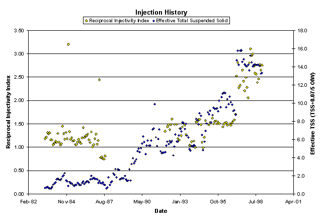
Figure 7. The Reciprocal Injectivity Index was then calculated and plotted along with an effective total suspended solids parameter. The RII shown here was based on reservoir pressure and the effect total suspended solid was defined as TSS+0.14 x OIW (see PEA-23 relationship). As can be seen, there is a reasonable correlation between the Reciprocal Injectivity Index and the water quality.

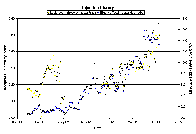
Figure 8. Reciprocal Injectivity Index and the effective total suspended solids history plot. The Reciprocal Injectivity Index shown here was based on the fracture pressure and the effective total suspended solids was defined as TSS+0.14 x OIW. As can be seen, there is a good correlation between the Reciprocal Injectivity Index and the water quality in the produced water injection portion. During early injection, aquifer water has a temperature of 20^oC or 70^oF, considerably colder than the reservoir (estimated to be about 200^oF). The poor correlation in the early injection stages may be due to thermal effects, which has not been considered in the calculation of the Reciprocal Injectivity Index. Consideration of thermal stress would reduce the fracturing closure pressures and thus increase the Injectivity Index (reduce RII).

Development of a PEA 23 Type Relation

One of the goals of this analysis was an evaluation of the legitimacy of the PEA-23 correlation in permeability ranges outside of those encountered at Prudhoe Bay from which the relationship was largely developed. It has always been acknowledged that the PEA-23 relationship was based on averaging of a large number of wells in regimes where the permeability was generally higher than encountered in this well.

The most difficult part of using the PEA-23 relationship is determining the Injectivity Index for clean water (II₀) at produced water temperatures and accounting for permeability effects. The following is the PEA-23 equation:

............................................................................................. (1)

where:

f(k) is a function of permeability defined in the PEA-23 relationship as:

................................................................................................... (2)

and WQ is a water quality parameter (from PEA-23) defined as

..................................................................... (3)

It should be noted that the permeability effect shown in Equation (2) was developed by Laurence Murray and others from permeabilities ranging from 20 md to 130 md. This relation may not apply to the very low permeability (between 0.5 md to 5 md) for this well. The following provides a method to estimate the permeability effect from the data for this well.

Taking the reciprocal of the equation (1) gives:

............................................................................................. (4)

or:

, or..................................................................................... (5)

................................................................................ (6)

where RII is the Reciprocal Injectivity Index.

Using the above relationship, it is now possible to obtain values for RII₀ and f(k) by plotting RII versus WQ. In this plot, a best fit curve yields the intercept (RII₀) and the slope (RII₀ x f(k)). This procedure was carried out and is demonstrated in Figure 9.

Once the Injectivity Index for "clean" produced water, II₀, and the permeability effect factor f(k) are determined, one can use these values in Equation (1) to predict the Injectivity Index for a given water quality, namely the total suspended solid (TSS) and the oil-in-water (OIW). Figure 10 is a comparison between the calculated Injectivity Index (II), calculated from the actual values of the injection rate and the pressure, and the predicted II based on Equation (1).

Referring to Figure 10, since the aquifer water (injected at early times) had a much lower temperature, thermal stresses should reduce the fracturing pressure. If thermal stresses were considered and lower fracturing pressures were used for the early cold water injection, the calculated Injectivity Index for the aquifer injection should be larger than what is shown in the plot.

Figure 11 is a comparison of the calculations. Again, if thermal stresses were considered and lower fracturing pressures were used for the early cold water injection, the calculated Injectivity Index for aquifer injection should be larger than what is shown in the plot. Although it is not done in this plot, the thermal stress effect could be estimated from Young’s Modulus.

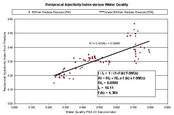
Figure 9. Reciprocal Injectivity Index (based on the fracturing pressure) versus the water quality, defined as 0.05TSS + 0.0007OIW from the PEA 23 relationship. The intercept yields the Injectivity Iindex of "clean" water at the produced water temperature. The slope gives the permeability effect factor for the permeability of this injector, which was estimated to be between 0.5 md and 5 md. The best curve-fit gives II₀ = 10 and the permeability effect factor f(k) = 4.4.

Figure 10. Comparison between the calculated Injectivity Index (II), based on the injection rate and pressure data, and the predicted II based on the PEA 23 relation shown in Equation (1).

The permeability factor used in Figure 11 is f(k) = 4.4, versus f(k) = 22exp(-k/22) = 19 (PEA-23) - for an assumed mean permeability of 3 md. The permeability effect equation f(k) = 22exp(-k/22) was based on data from permeabilities between 20 md and 130 md. The estimated permeability of 0.5 to 5 md for this injector is certainly much smaller, and the discrepancies are not unexpected.

Similar observations are made when evaluating Figure 12, which is analogous to Figure 11 with the exception that the produced water portion only is plotted.

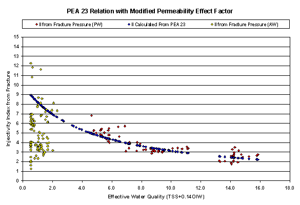
Figure 11. Comparison between the calculated Injectivity Index (II), based on injection rate and pressure data, and the predicted II based on the PEA 23 relationship with a modified permeability effect factor.

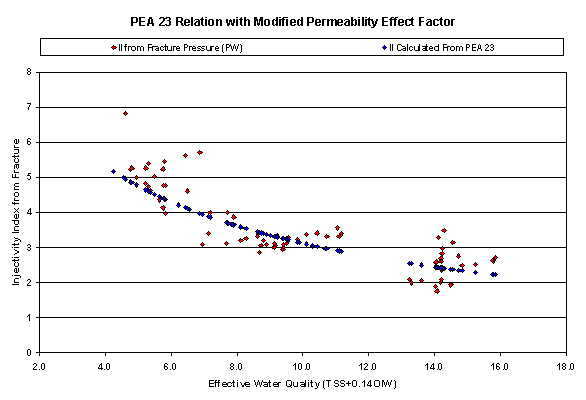
Figure 12. Comparison between the calculated injectivity index (II), based on injection rate and pressure data, for the portion of produced water injection only and the predicted II based on the PEA 23 relationship with a modified permeability effect factor. The permeability factor used in this plot is f(k) = 4.4, versus f(k) = 22exp(-k/22) = 19 for a mean permeability of 3 md. The permeability effect equation f(k) = 22exp(-k/22) was based on data from permeabilities between 20 md and 130 md. The estimated permeability of 0.5 to 5 md for this injector is certainly much smaller.

Conclusions and Recommendations

Based on data analyzed here in this document and data analyzed and reported in two previous documents (distributed to Jean-Louis Detienne), it concluded that

· The PEA-23 relation works reasonably well for data that were analyzed.

· Permeability has a large effect on the relation.

· The permeability effect equation of f(k) = 22 exp(-k/22), in the original PEA-23 relation, was derived for permeabilities varying from 20 md to 130 md. This equation does not, as expected, work for low permeability formations.

· Based on the data analyzed here, permeability effect for low permeability formations is less.

· Method was proposed and used here, based on the interception and slope of linear curve-fit, to obtain the two important parameters - the injectivity index for clean water and permeability effect factor, in the PEA-23 relation.

· PEA-23 relation is used for predicting water quality effect on injectivity. Temperature effects are not considered in this relation and it is recommended to eliminate temperature effect in the data analysis process. For example, in order to eliminate temperature effect on the injectivity index of clean water at produced water temperature, it is recommended to follow the method proposed here.