Analysis of Stimulation of Fractured Injector (Maersk Field A)

Introduction

This is a chalk reservoir with a permeability of only a few md. Injectivity decline was observed on a number of the water injection wells and an acid stimulation campaign was conducted on more than a dozen injectors. Stimulation results for twelve injectors were analyzed. Some of the treatments were bullhead acidizing (15% HCl) and others were on-the-fly acidizing (1.5 to 2% HCl). Correlations were attempted to relate the after-stimulation injectivity and the injectivity decline rate to pre-stimulation injector performance and damage. These correlations were applied to forecast initial after-stimulation injector performance and to estimate how long the injectivity enhancement would last. These forecasts are necessary input for stimulation design and for payback time estimates. Bullhead acidizing only yielded a slightly better stimulation performance than on-the-fly acidizing.

The objectives of this case study were:

· To investigate the impact of the acid delivery methods on stimulation effectiveness.

· To develop correlations for predicting injectivity enhancement and the post-treatment injectivity decline rate.

· To assess if the knowledge developed from stimulation analysis for some of the injectors could be applied to other injectors for forecasting stimulation performance.

Water Source and Quality

"The field gets some 75% of all PW from the separation process resulting in the injection water being mainly SW." However, there are no data for each individual injector concerning the mixing ratio of the produced water and seawater portions. The water temperature at the wellhead, for one well, is shown in Figure 1.

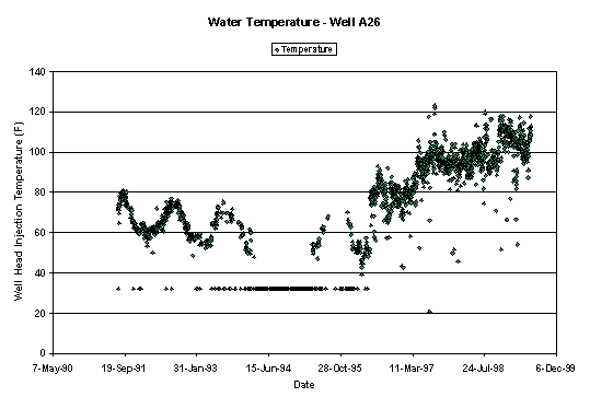
Figure 1. Wellhead temperature history. The temperature was initially between 60 and 80°F. Starting in the summer of 1996, the water temperature began to increase gradually to over 100°F. This temperature increase is assumed to be due to a gradual increase in the produced water portion of the water blend that was injected.

Water quality data are also available (Figure 30). This is one of the few cases of data analysed from various operators where acceptable, continuous water quality information was available. For appropriate quantitative analysis, a recommendation is some form of regular measurement of the characteristics of the injected water.

Typical Analyses

The analysis methodology for this field is demonstrated in the accompanying figures. Relevant details are indicated in the individual figure captions.

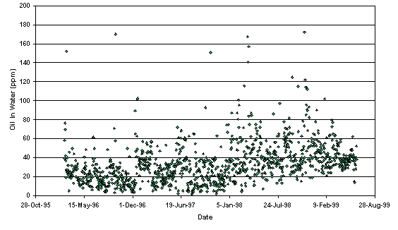
Figure 2. Oil-in-water versus time. The oil-in-water concentration increases gradually with time. This is consistent with the assumption that the portion of produced water increases with time. This assumption is also consistent with the wellhead injection temperature (Figure 1).

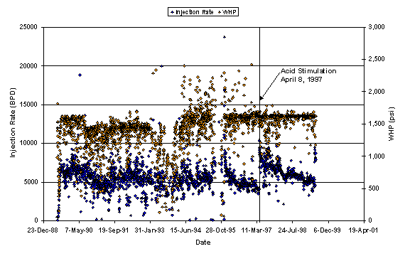
Figure 3. Wellhead injection pressure and injection rate history plot. Two clear features can be seen from this plot - there was an increase in wellhead pressure beginning in the summer of 1994 and there was an obvious increase in the injection rate right after acid stimulation. There was also an obvious increase in the injection rate towards the end of 1995. It is suspected this was due to shut-in and restart of the injector as there was a period of 2 months of missing data.

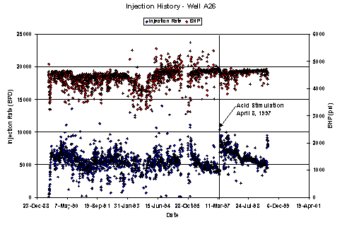
Figure 4. The first step in any analysis is to convert surface information to formation face data. Bottomhole injection pressure and injection rate are shown in this plot.

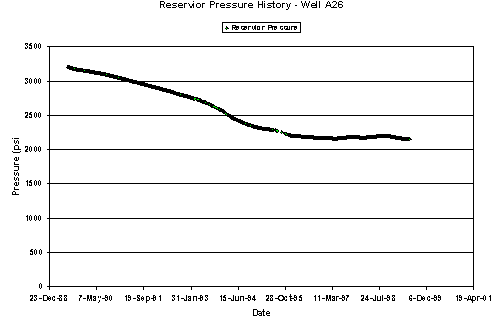
Figure 5. Reservoir pressure as a function of time. There are over 2 months of missing data between August 1995 and October 1995. The second step in any reasonable analysis is to ensure that you understand the average reservoir pressure.

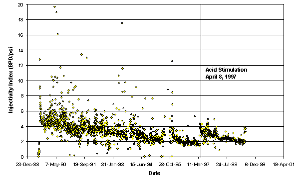
Figure 6. The next step is to look at basic performance. The most convenient initial method is to look at Injectivity Index. This plot shows the Injectivity Index as a function of time. As can be seen, there is a clear benefit of acid stimulation – the Injectivity Index increases after the treatment and the benefit was sustainable for a reasonable period of time.

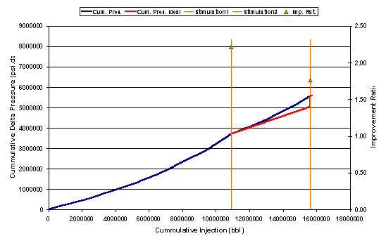
Figure 7. Next look at the Hall plot. Plot the conventional Hall plot information. Superimpose an ideal Hall plot immediately after the treatment and extrapolate this ideal situation ahead in time (assuming no further damage after stimulation). Calculate the improvement ratio for the treatment (ratio of the Injectivity Index after the stimulation to that before stimulation). There is a clear benefit to the stimulation in this situation. The benefit is sustainable (does not deviate from the ideal Hall plot) for quite some time.

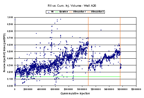
Figure 8. Now look at the Reciprocal Injectivity Index versus the cumulative injection volume. Performance degradation between stimulations is evident and the trends appear to be nearly identical!

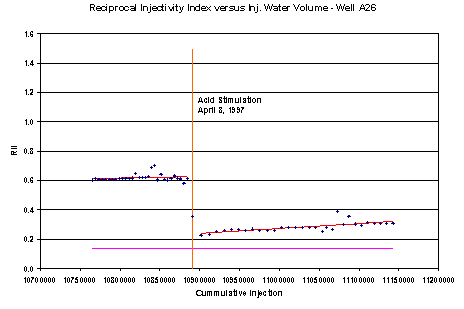
Figure 9. Curve fit the RII data. A thirty-day linear fit was used to define the Improvement Ratio and the slope - to describe how fast the stimulation benefits will diminish. The Improvement Ratio is the ratio of the intercepted Injectivity Index after stimulation to the intercepted Injectivity Index before the stimulation. Figure 38 is a similar example.

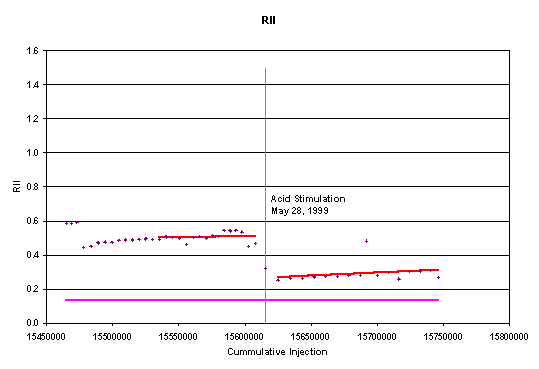
Figure 10. Reciprocal injectivity index versus cumulative injection volume near the stimulation on May 28, 1999. A thirty-day linear fit was used to define the Improvement Ratio and the slope - to describe how fast the stimulation benefits will diminish. A good stimulation yields a relatively high Improvement Ratio and a small slope after stimulation.

Correlations?

Stimulation data from a dozen wells were analyzed. Both bullhead acid stimulation and on-the-fly acid stimulation data were available for some of the wells. Correlations were developed to estimate post-stimulation performance from pre-stimulation information. The objectives of this analysis were to predict the following before a stimulation is performed on a well:

· How much improvement in injectivity will be due to a stimulation?

· How long the improvement will last?

Injector performance just before and just after the stimulation may be approximated by linear lines as shown, for example, in Figure 38. The Improvement Ratio is defined as the ratio of the Injectivity Index after the stimulation to the Injectivity Index before the stimulation. The Injectivity indices are determined from the intersection values. Recall that DRII is defined as:

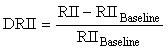
where the RII is the intersection value (on the stimulation line) of the Reciprocal Injectivity Index.

· A smaller Injectivity Index before stimulation results in a larger Improvement Ratio. The lower the injectivity, the greater the relative improvement.

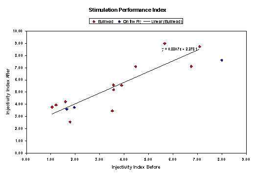
Figure 11. Injectivity Index before and after the stimulation on April 8, 1997 for a number of wells where acid was bullheaded or injected on-the-fly into the fractures.