Horizontal Injection Wells - Best Practices for Modeling

Contacts

Tony Settari

ASettari@TaurusRS.com

Taurus Reservoir Solutions

Key Issues

1. Adequate consideration of thermal stress effects is essential.
   
2. It is necessary to correctly incorporate thermal PVT effects.
   
3. Consider the necessary gridding issues.
   
4. Properly represent fracture(s).

Relevant references are cited.

Thermal Stress Effects

Recommendation 1.1: Always use a thermal reservoir simulator to model injection into horizontal wells.

There are two major reasons why simpler isothermal modeling may give misleading results for PWRI injectors:

1. Cooling the fluids around the wellbore produces oil and water viscosity changes. Even for small temperature differences between the injected and in-situ temperature, the effect can be large. Ignoring the viscosity effects will overpredict well injectivity and if one is matching history, will lead to using more damage to compensate.

2. Cooling produces thermal stresses around the wellbore which will alter the conditions for fracture initiation and lower the fracture propagation pressure. In addition, if one considers stress-dependent permeability and porosity, these will also be affected. Again, thermal stresses may be small in a very soft formation, but since that implies very high permeability, pressure gradients and poroelastic stresses will also be small and therefore the thermal effects will still be significant.

   Modeling of a horizontal Prudhoe Bay injector with a model that uses constant fluid viscosities at in-situ temperature produced large injectivity and bottomhole pressures never reached fracturing conditions during the first 45 days of injection. However, in reality, the actual recorded field data for this well definitively indicated fracturing within 2 days of injection. These simulation results were obtained even though the effect of thermal stresses was accounted for and the failure to adequately represent the onset of fracturing was due entirely to the fact that the model did not simulate reduced fluid mobility associated with injection of a cooler fluid.

Back to Key Issues

Recommendation 1.2: Accurately estimate and simulate bottomhole injection temperatures - BHT directly affects thermoelastic stress changes.

• Investigate the significance of thermal stresses based on a first estimate of bottomhole temperature and the use of WellStress (a Toolbox component for inferring poro-themroelastic stress effects).
• Thermal wellbore flow software can be used to account for heat transfer from the surface to the injection zone(s), based on rate, surface temperature, thermal gradient, pipe size, etc.
• It may be appropriate to have downhole temperature measurements for a typical well, in order to build a field-wide correlation between injection rate, injection temperature and bottomhole temperature.
• Coupled thermal wellbore hydraulics modules, linked to a reservoir simulator (this kind of modeling is quite specialized and not widely available - paper SPE 59453 describes such a model) can be used.

Typically, the reservoir simulator will require the bottomhole temperature for the injection well. The experience gained in the modelling of a Prudhoe Bay horizontal injector has shown that one of the key factors in accurately matching the observed data is having accurate BHT for the injector. The thermoelastic stress changes due to injecting produced water that has cooled at surface can be significant, considering the depths of some of the injection zones. The modelling showed that a difference between the bottomhole injection temperature and the reservoir temperature of about 100°F caused the thermal stress effects to dominate. This temperature difference caused the minimum principal stress to decrease from an initial value of ~6000 psi to the propagating fracture pressure of ~5300 psi. The modelling considered both poroelastic and thermoelastic stresses with an overall decrease indicating a dominating thermal effect.

Back to Key Issues

Recommendation 1.3: Accurately measure or sensitize the expected range of the thermal expansion coefficient - this directly affects thermoelastic stress changes.

• If possible, obtain laboratory measurements of the thermal expansion coefficient of the reservoir material.
• If laboratory data are not available, estimate the thermal expansion coefficient from published data and sensitize the effects to the potential error band of that data. One published source of this information is the SPE Mongraph by M. Pratt.

In reservoirs where thermoelastic effects dominate, the stress changes caused by the temperature gradients are significant. The magnitude of these stress changes largely depends on the material's thermal expansion coefficient. The measurement of the thermal expansion coefficient is reasonably simple and, therefore, this parameter can be quantified to eliminate a further source of modelling error.

Back to Key Issues

Recommendation 1.4: Conduct a detailed analysis of the rock mechanics behaviour of the reservoir material - in particular for sharp thermal gradients.

• Infer the stress paths of the regions subject to the largest stress changes using laboratory data and field measurements.
• Identify the failure envelope of the material (shear as well as compaction) as this may be important for creating a dilation zone around fracture as well as compaction ring.

Sharp thermal (as well as pressure) gradients, potentially present when injecting under fracturing conditions, can cause elevated deviatoric stresses which may induce shear or compaction failure of the matrix material. This failure can cause changes in the pore structure, which in turn will affect the injectivity of the well. Identification of these effects may be possible using pressure transient analysis (PTA) with coupled modelling to identify the potential for changes of injectivity due to failure in the matrix surrounding the fracture.

Back to Key Issues

Thermal PVT Effects

Recommendation 2.1: The thermal dependence of fluid viscosities becomes important when you are injecting at temperatures different from the reservoir temperature.

There are two major reasons why simpler isothermal modeling may give misleading results for PWRI injectors:

• Cooling the fluids around the wellbore produces oil and water viscosity changes. Even for small temperature differences between the injected fluid and in-situ temperature, the effect can be large. Ignoring viscosity effects will overpredict well injectivity, and, if you are matching history, this will lead to using more damage to compensate.

• Cooling produces thermal stresses around the wellbore. This will alter the conditions for fracture initiation and lower the fracture propagation pressure. In addition, if one considers stress dependent-permeability and porosity, these will also be affected. Again, thermal stresses may be small in a very soft formation, but since that implies very high permeability, pressure gradients and poroelastic stresses will also be small and therefore the thermal effects will still be significant.

  Modeling of a Prudhoe Bay horizontal injector with a model that used constant fluid viscosities (viscosities specified at the in-situ temperature only) produced large injectivity and bottomhole pressure was simulated to never reach fracturing conditions during the initial 45 days of injection. However, the models that were used to simulate this well with temperature-dependent viscosities indicated fracturing within 2 days of the start of injection, in agreement with field data (Figure 1). This significant difference in simulation results was obtained even though the effect of thermal stresses was accounted for equally in both of the models that were used (Figure 1).

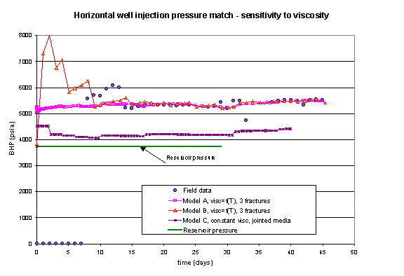
Figure 1. Effect of temperature-dependent viscosity on the predicted injection pressure. Notice that the simulator that did not account for changes in viscosity underestimated the injection pressure because the mobility was too high.

• A good description of viscosity behaviour of in-situ fluids, as well as tdhe injected fluid(s), is needed to accurately model the injectivity effects associated with mobility ratios.
• A thermal model should be used whenever possible even if the model is uncoupled (i.e., does not include stress modeling).

The above modelling comparison (for the horizontal injector that was selected for analysis) showed the importance of including the thermal dependence in the viscosity behavior of the in-situ and injected fluids. The injectivity predicted by the model that neglected thermal effects was too high, primarily because the mobility of the in-situ fluid remained too high - it was based solely on the initial reservoir temperature. The effects of cooling were noticeable, causing the mobility ratio to change and the injectivity to decrease, such that fracturing pressures were attained more quickly, when simulation was carried out with models that incorporated appropriate viscosity dependency.

Back to Key Issues

Recommendation 2.2 The PVT of the in-situ fluids cannot be overly simplified. It must include as a minimum the black-oil representation if there is production near the injector well and pressure may fall below bubble-point.

• Include the full black-oil PVT if the pressure may drop below the bubble point pressure somewhere near the horizontal injector.

  The model of the horizontal injector that was analysed also included several producing wells to balance the voidage for a sector of the field. The modelling showed the importance of including the full black-oil PVT in the modelling since the producing wells created a drawdown zone with pressure falling below the bubble point pressure. Once this occurred, the viscosity of the in-situ oil increased and the overall mobility of the system dropped. Simplification of the in-situ fluid to a single phase, constant viscosity medium was also identified as a reason why simplified modelling verestimated the injectivity of the system, with direct implications on the predicted bottomhole pressure response.

  An example of the range of answers generated by various (seemingly reasonable) simplifications of the PVT is shown in Figure 2. Obviously, such differences may render a history match done with simplified PVT completely meaningless.

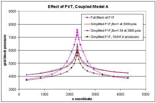
Figure 2. Effect of PVT simplification on the pressure gradients that are calculated around the well.

Back to Key Issues

Gridding Issues

Recommendation 3.1: Use sufficient grid refinement around the well - a grid sensitivity "experiment" may be necessary.

• Make the grid size of the cell containing the well approximately 2 to 5 times the wellbore diameter.
• Use an increasing grid size away from the well (in the plane perpendicular to the well direction) in some (usually logarithmic) fashion.

  Calculated injection pressures can be extremely sensitive to the grid size around the well, especially when sharp temperature gradients exist. While the best solutions are offered by non-structured embedded grids, these are not yet in common use and you usually must construct a Cartesian grid in the plane perpendicular to the well direction. If in doubt, it is always possible to conduct a grid refinement experiment to ensure adequate accuracy. In coupled flow and stress simulations, the resolution of the stresses around the well is also highly grid-sensitive.

Back to Key Issues

Recommendation 3.2: If possible, eliminate the significance of the well index in the simulation.

• It is preferable to refine the grid so that the well index, WI, becomes very large and therefore the pressure drop between the block pressure and BHIP becomes insignificant. If Peaceman's formula is used for WI (which is standard in simulators), this will occur when the grid size is about 5 times the wellbore diameter. Reducing the grid size further would result in negative WI and the software will generally not allow the model to run.

• If further grid refinement is necessary for other reasons, you can "trick" the simulator to accept smaller grid sizes by either using an artificially smaller well radius or by introducing artificial (positive) skin. In either case, ensure that the well index is very large.

Note 1: The formula normally used to compute WI for a horizontal well in the x-direction, with a well radius r_w, in a given cell with dimensions of dx, dy and dz, is (Reference 2):

WI = 2pk_avgdx/(ln(r₀/r_w + S) ............. Equation (1)

where:
S is the skin and r₀ is the Peaceman radius. In the usual case of permeability anisotropy with k_H and k_V, the k_avg and r₀ are given by:

k_avg = (k_Hk_V)^1/2

r₀ = 0.28[(k_Hk_V)^1/2dy² + (k_Vk_H)^1/2dz²)/[(k_Vk_H)^1/4+ (k_Hk_V)^1/4]

Therefore, if your choice of gridding renders WI negative, you can adjust either r_w or use artificial skin to give the term ln(r₀/r_w + S) a small positive value.

Note 2: The skin in Equation (1) is not the total skin for the well. If the grid is fine, this is possibly not even the entire completion skin. Also, the external radius is different so the skin in the II equation must be recalculated References 3 and 4).

Back to Key Issues

Fracture Representation

Recommendation 4.1 Use other tools developed in the PWRI to determine from historical data if fracturing is taking place. If simulating a project without history, decide if injection at fracture pressure is part of the strategy.

• Use, for example, the methodologies developed for soft formations evaluation to identify initiation and extension of fracture(s) from p vs Q plots, Hall plots, etc.
• Confirm your conclusions by determination of the original fracture pressure from initial stresses, and correcting for poroelastic and thermoelastic stresses (e.g., by using the WellStress tool [in the PWRI Toolbox], although keep in mind that this tool is intended for vertical wells).

Back to Key Issues

Recommendation 4.2: If fracturing is important, use a coupled reservoir and fracture simulator - if possible.

• Align the grid so that the intended plane of fracture propagation is in a grid plane.
• Approximation using a stationary fracture can be done by modifying the flow transmissibilities in the fracture plane. This will generally overestimate the injectivity early and, depending on the chosen length, underestimate the injectivity at late times. Better results are obtained if the simulator allows modification of the fracture transmissibilities with time, but this requires predicting fracture propagation using a separate means (e.g., fracture model).

Back to Key Issues

Recommendation 4.3: In coupled fracture modelling, use the strongest degree of coupling that is available.

When using a coupled fracture model, solving the fracture propagation in large time intervals may "delay" fracture propagation and introduce errors in the computed injection pressure.

• If possible, use one-to-one coupling, i.e., solving the fracture propagation for each time step of the reservoir model.

The effect of solving the fracture propagation only occasionally is shown on Figure 3. Other issues important for fracture coupling are discussed in Reference 5.

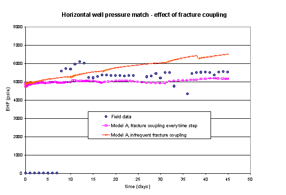
Figure 3. Effect of the frequency of the fracture coupling on the predicted injection pressure.

Back to Key Issues

References

1. Stevens, D.G., Murray, L.R., and Shah, P.C.: "Predicting Multiple Thermal Fractures in Horizontal Injection Wells; Coupling of a Wellbore and a Reservoir Simulator," Paper SPE 59354, 2000 SPE/DOE Improved Oil Recovery Symposium, Tulsa, Oklahoma (3-5 April 2000).
2. Peaceman, D.W.: "Interpretation of Well-Block Pressures in Numerical Reservoir Simulation with Nonsquare Grid Blocks and Anisotropic Permeability," SPEJ (June, 1983), pp. 531-543.
3. Odeh, A.S. (check initials): "The Proper Interpretation of Field Determined Buildup Pressure and Skin Values for Simulator Use," paper SPE 11759 (1985).
4. Settari, A.: Advanced Reservoir Simulation, manuscript, to be published by Elsevier (2002).
5. Settari, A.: "Coupled Fracture and Reservoir Modeling," Proceedings of the Three Dimensional and Advanced Hydraulic Fracture Modeling Workshop, 4th NARMs Symposium, Seattle, Washington (July 29, 2000) pp. 71-77.

Back to Key Issues

Top

Previous

Fracture Models Summary

Documents