Microseismic Measurements
Introduction:
Microseisms are generally seismic energy emitted by shear slippage along weakness planes in the earth (Figure 1). When slippage occurs, seismic energy is released.
|
Figure 1. When a hydraulic fracture (for stimulation or PWRI) is created there are local increases of stress and pore pressure - due to leakoff and poroelastic effects. Fluid entering natural fracture systems can increase the pore pressure in these, leading to a reduction in the effective stress normal to the fracture surface and causing the fracture faces to slip - the shear stresses acting along the surface of the fracture are not reduced by the pore pressure but the effective normal stress is. Because the effective normal stress is smaller, the frictional resistance along the fracture is smaller and the fracture faces can slip past each other. The analog to consider is the amount of effort required to push a block of material across a table if you are pressing down hard ("high effective normal stress") versus if you are pressing down with less force ("low effective normal stress").
|
When slippage occurs, both compressional waves (P waves) and shear waves (S waves) are emitted. The wave velocities are different - P waves travel faster than S waves. These waves are detected at a triaxial receiver (Figure 2).
|
Figure 2. P waves and S waves are emitted when slippage occurs. These waves are detected at strategically placed triaxial receivers. Compressional waves have a higher velocity than shear waves.
|
Where are the Receivers Placed?
The microseisms that are generated as a result of injecting into a hydraulic fracture are quite weak. Receivers placed at the surface are, in most cases, too far away to reliably detect these signals. On the other hand, if sensors are placed close to the injection zone in the well that is being injected into, there is too much noise from the pumping operations themselves (Figure 3).
|
Figure 3. P and S waves are difficult to detect if the receivers are at the surface. If the receivers are in the injector itself, there is too much noise.
|
This necessitates placement in offset wells. If a single offset is used, the receivers need to be logically placed - you need to have a preconception of where the fracture will be going. If receivers are placed in more than one offset well, they should similarly be situated to maximize coverage across what you visualize will be the trajectory and vertical extent of the hydraulic fracture in the injector. Refer to Figure 4.
|
Figure 4. Receivers can be placed in one or more offset wells.
|
Single Well Mapping
The distance to, and the elevation of the originating slippage event are determined from the arrival times measured at the receivers (Figures 5 and 6). The direction to the event is discriminated from the P-wave particle motion. Remember that these microseisms are small amplitude and high frequency and that the receiver distance will be a typical interwell spacing. As such, high quality receivers are essential.
|
Figure 5. Receivers in a single offset well.
|
|
Figure 6. Typical microseism traces. The center waveform shows P and S wave arrivals.
|
The receivers automatically detect the events and process the signals. Location processing uses either:
-
A Homogeneous Model: Joint P-S Distance Regression, or,
-
A Layered Model: Vidale/Nelson Algorithm.
The additional information that is required for processing the data includes:
-
Formation Velocity: This can be determined from techniques such as using an "advanced" sonic log (P and S Waves) or from a crosswell survey.
-
Receiver Orientation: This can be determined from signals acquired when the injector is perforated, or with an air gun or other source (full interval scan).
-
Surveys: Well-to-well location needs to be established from surface surveys and deviation surveys.
Procedures
For a stimulation fracturing treatment, typical procedures would be:
-
Prior Day: This would provide the opportunity to mobilize and set up the site. Receivers have already been installed in one or more offsets. These receivers are oriented with check shots (e.g., air gun or perforations). Background monitoring is carried out.
-
"Frac" Day: Monitoring is carried out before, during and after the treatment. Many of the events may occur after shut-down. Real-time or near-real-time processing is available before demobilization.
Limitations
There are some current limitations for this technology:
Microseismic Interpretation
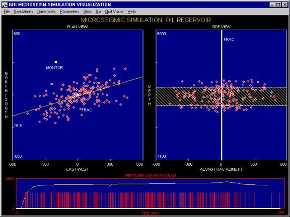
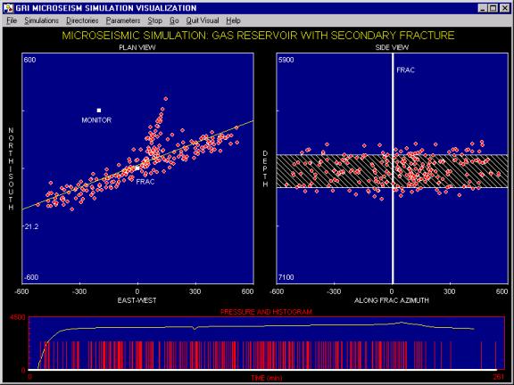
Microseisms originate in an envelope around a hydraulically induced fracture. This envelope provides indications of the height, length, azimuth and indicates any asymmetrical growth characteristics (i.e., may grow more in one direction than another - up dip for example). The events that you are dominantly seeing are fluid loss indiced slippage in fractures around the main treatment. Figure 7 is a schematic example. The response of the formation around the fracture depends on the compressibility of the native fluid. In a reservoir with a compressible fluid, Figure 8, the pressure in the "remote" fractures is altered only locally to the mother fracture system. In a reservoir with a slightly compressible fluid (oil or injected water) pore pressure alteration around the fracture extends farther away (Figure 9).
|
Figure 7. The microseismic events that you usually see are not explicitly associated with the fracture itself. They are commonly due to slippage in pre-existing (and maybe newly created) shear fractures away from the fracture.
|
|
Figure 8. If the reservoir contains a compressible fluid, poroelastic effects indicate that the compressibility of the fluid in the formation will quickly swallow up changes in the pore pressure in natural fractures. The events that will occur, due to increases in pressure in the native fracture systems, will be close to the main fracture.
|
|
Figure 9. In a formation containing relatively incompressible fluid - i.e., you have been injecting produced water for a significant period of time, the pressure will be altered farther away from the mother fracture and the envelope defining the fracture will extend deeper into the formation.
|
Remarkably large displacements occur for substantial distances away from large hydraulic stimulation fractures. Figure 10 is one example.
|
Figure 10. Full poroelastic modelling of a hydraulic fracture shows significant displacements perpendicular to the surface of the fracture. There are shearing events that accompany these displacements.
|
Field Examples
Historical data are available that indicate that long term waste and oilfield injection operations can result in large destabilized areas around the injector, with moderate earthquakes (a consequence of slippage) detected at the surface. (refer, for example to Nicholson, C., and Wesson, R.L., 1990, and "Earthquake Hazard Associated With Deep Well Injection -
A Report To The U.S. Environmental Protection Agency," USGS Geological Survey Bulletin 1951).
Figure 11 shows example signals recorded during hydraulic fracturing at the LANL Hot Dry Rock Project site. It was attempted to grow a hydraulic fracture from one well to another. Approximately 6,000,000 gallons of water were pumped at rates of 50 bpm.

|
Figure 11. LANL had a hot dry rock geothermal project site in the Jemez cauldera, near Los Alamos, New Mexico. For the pilot, it was desirable to have a conduit to flow fluid from one well to another. During the hydraulic fracturing operations that were attempting to communicate the two wells, microseismic events were monitored. The trace of the system is well delineated and microseismic events engulfed the targeted well. However, as testimony to the complexity of the created fracture networks, only poor communication was developed between the injection and the producing well.
|
Figure 12 is another hot dry rock example. This one is from the Cambourne School of Mines pilot in the UK.
|
Figure 12. Microseismic events measured during injection at the Cambourne School of Mines pilot. A progressively evolving linear trend is evident in these side views.
|
Figure 13 shows microearthquakes detected during injection in the San Andres Field.
|
Figure 13. Microseismic events measured during injection in a LANL program in the San Andres Field.
|
Methodology for Microseismic Monitoring
-
Monitor Initial Injection Behavior: The fracture is imaged and an azimuth is inferred.
-
Examine Attributes Of Late-Time Behavior: Look for clustering and linear trends. High stress relief is associated with tip microseisms and low stress relief is associated with leakoff microseisms. There are some field cases where microseismic measurements have been validated by other monitoring techniques. The work at the M-Site is one example. Downhole tiltmeters measured deformation - this allowed a supplementary measurement of the fracture height. There was some control on the length of the fracture because it was specifically determined that the fracture intersected a lateral well that was 287 feet from the treatment well. The azimuth was further defined by the intersection with another lateral well; this lateral was 135 feet from the treatment well. These controls are shown in Figure 14. Figure 15 is a plan view of some of the microseismic events recorded during operations at the M-Site.
|
Figure 14. The M-Site was a field laboratory in the Piceance Basin. There were two monitoring wells and the fracture (shown schematically in red) intersected both of these wells.
|
|
Figure 15. A plan view of some of the microseisms recorded during operations at the M-Site field laboratory. Figures 16 through 18 show time lapse representations of microseisms during stimulation in one zone at the M-
Site. Figures 19 through 22 are another example.
|

|
Figure 16. Plan and elevation views of recorded microseimic events - Time 1.
|
|
Figure 17. Plan and elevation views of recorded microseimic events - Time 2.
|
|
Figure 18. Plan and elevation views of recorded microseimic events - Time 3 - notice the fracture running off in a spur.
|
Additional Information
For additional information, abstracted publications are also available. The technology is at a point where subsurface imaging can be an important capability for process monitoring, optimization of injection procedures and regulatory compliance. The technology is now at a level where microseismic diagnostics can be applied. This is becoming progressively more true with development of advanced receivers, improvements in fiber optic telemetry, improved processing hardware and software and improved appreciations of reservoir structural behavior.
<
Summary
References
>