Examples
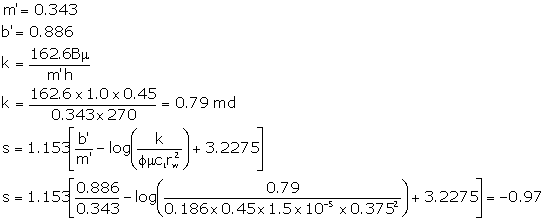
Figure 16 shows an example data set. There is an inflection point at a surface pressure of 1,000 psi. For illustrative purposes, assuming no friction, a depth of 7260 feet and a fluid pressure gradient of 0.433 psi/ft, 1000 psi gives an estimated fracture opening/reopening pressure gradient of 0.57 psi/ft. The data can be further analysed for formation properties using multi-rate analysis methods. This is shown in Figure 17. The first four points fall on one curve, indicating pseudo-radial flow.

In Figure 17, the higher rate points do not fall on a straight line because the assumptions of radial, infinite acting flow are no longer satisfied, since fracturing has occurred.
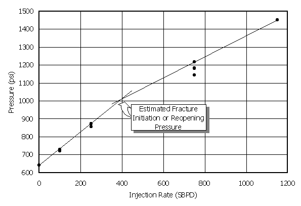
Figure 16. An example step-rate analysis (reported in Earlougher, 1977, and originally from Felsenthal, 1974). The multi-rate plot for these data is shown in Figure 17.
An Excel file (for the foregoing example) is attached (click button below), indicating how multi-rate analyses are carried out.
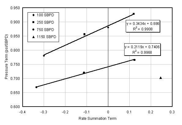
Figure 17. Multi-rate analysis for the data set shown in Figure 16.
Figures 18 and 19 show rate and processed step-rate data from PCP Rosemary 16-07-22-16W4. Only surface data were used in this evaluation. No information was available on the times for each injection stage. A parametric variation in times was implemented. Three cases are shown. The first is for arbitrary equal times. There is no consistent or interpretable behavior. The pressure data are not clarified at all and it is still difficult to infer a fracture opening pressure. This may have been the real situation and there could have been a gradual transition from radial to linear or bilinear (fractured) behavior. Or, possibly the time steps became shorter for each subsequent injection stage. An arbitrary example is shown by the red circles in Figure 19. Two straight lines can be delineated, indicating a surface fracture opening pressure of 6.03 MPa. Finally, another situation is arbitrarily assumed. The first three stages were taken to be at relatively long injection times and all following stages were short. This gives a dramatically different signature that is relatively meaningless. If injection times were available, some of the uncertainty in this data set could be removed (i.e., in Figure 18, can a discreet fracture opening/reopening pressure be determined by processing the data and accounting for previous response in the reservoir?). Figure 19 shows that, incorporating time effects and being consistent in the performance of each injection cycle could make a significant difference in interpretation of the data. Time information is not available for this case, so no improved interpretation is possible. The example is shown strictly to indicate the importance of accounting for the duration of each injection stage.
This is not an academic exercise. It is intended to demonstrate:
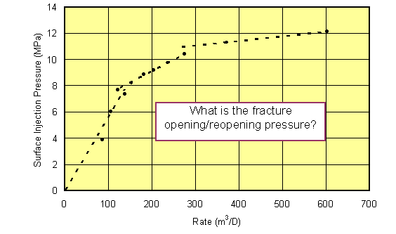
Figure 18. Raw, surface step-rate data from PCP Rosemary 16-07-22-16W4. It is difficult to determine a distinct reopening pressure - either because of frictional effects, variable injection time effects, reopening of a conductive fracture or even more complicated fracture growth behavior. Multi-rate analysis can help to remove some of the uncertainty.
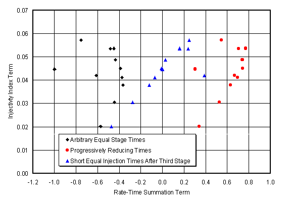
Figure 19. Arbitrary processing of surface step-rate data from PCP Rosemary 16-07-22-16W4, showing the influence of different injection stage times. The recommendation is that uniform time steps should be used and that multi-rate evaluations are important for discriminating behavior.
More Rigorous Evaluation of SRTs
SRT data actually contains much more information than what is used in the techniques described above, both about reservoir and fracture properties. However, to access this information it is necessary to:
Analysis Below Fracture Opening Pressure
Each step below the fracture initiation/opening/reopening pressure is a transient event. There is a large slope initially and a small slope at the end of a constant rate. Only the end point is used in graphical analyses. Simulation of the early stages can be carried out with conventional models and early and late slopes can be matched. These matches will yield both kh and system compressibility. The simulation can incorporate any known wellbore skin components.
When the simulation starts to deviate from the data, this is an indication of induced fracturing, or increasing conductivity of a pre-existing fracture. At this point, the conventional model cannot give any more detailed information, beyond indicating the approximate position of departure.
Analysis Above Fracturing Pressure
Coupled fracture-reservoir modeling is required at this point. These can be models using fracture mechanics principles, partially coupled (e.g., GEOSIM, with fracture coupling) or fully coupled (BP's model, after Clifford, et al.). The process can be also modeled as re-opening of joints or creating a high permeability channel (Visage, or GEOSIM with stress-dependent fracture representation).
Simultaneous matching of the rate steps and the falloff (while keeping the reservoir properties from the match below fracturing pressure) allows estimation of:
The estimate of the undisturbed minimum stress will generally differ from the graphical method result and can be lower for a multitude of reasons.
The pre-existing fracture can be incorporated in the simulation analysis and will generally result in more gradual change of the slope, as seen on the Rosemary example.
In general, simulation analysis can give clear answers in some complex cases that cannot be interpreted by the graphical methods. However, this is achieved at a considerably higher effort.
The first step is to look at basic radial flow relationships and see if radial flow at the low rates makes sense. The first step is graphical.
The second is to match the low and high rate ends with analytical models to look at the two limiting situations, with and without a fracture. If there is a deviation from low rate prediction and the actual data (in the right direction) it indicates a good test.
The final step, if warranted, is numerical analysis to make all parts fit together.
It is important to take into account pre-existing fractures. For matching pressures below pfoc, (closure pressure) determine the reservoir permeability and the fracture conductivity and forecast to higher rates. The point of departure between this theoretical curve and the measured data is an independent measure of the value of pfoc. Above pfoc, it is necessary to iterate with a fracture model to match the measured data.
Some operators evaluate SRT with spreadsheet models that have a radial flow and a fracture flow component.
| <Analysis | Methods> |
|
|
|
|
|